1.1: Defining a Limit
We base all topics in calculus on one important topic—the limit. Limits are a fundamental tool that enables us to describe how a function behaves as we change its input. In this section we define limits and present numerical and graphical methods to investigate them. We discuss the following topics:
Definition of a Limit (Intuitive)
A limit is the number that a function \(f(x)\) approaches as
its input \(x\) approaches some number \(a.\)
If \(f(x)\) gets closer and closer to \(L\) as \(x\) gets closer and closer to \(a\)
(without necessarily being \(a\)), then we say
\[\lim_{x \to a} f(x) = L \pd\]
This notation is read as the following: The limit of \(f(x),\) as \(x\) approaches \(a,\) is \(L.\)
We could also use arrow notation
by writing \(f(x) \to L\) as \(x \to a,\) meaning \(f(x)\)
tends to \(L\) as \(x\) is made close to \(a\) (but \(x \ne a\)).
In other words, we can make the values of \(f(x)\) arbitrarily close to \(L\)—as
close to \(L\) as we please—by making \(x\) sufficiently close to \(a\) but not equal to \(a.\)
We will present a more precise definition in
Section 1.5,
in which we study the interpretation of the phrase as close to \(L\) as we please.
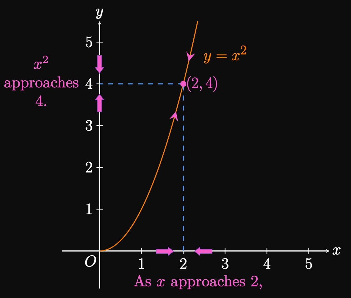
As an example, the following table shows values of \(f(x) = x^2\) for selected values of \(x.\)
| \(x\) | \(f(x) = x^2\) |
| \(1\) | \(1\) |
| \(1.5\) | \(2.25\) |
| \(1.7\) | \(2.89\) |
| \(1.9\) | \(3.61\) |
| \(1.99\) | \(3.9601\) |
| \(1.999\) | \(3.996\) |
| \(x\) | \(f(x) = x^2\) |
| \(2.001\) | \(4.004\) |
| \(2.01\) | \(4.0401\) |
| \(2.1\) | \(4.41\) |
| \(2.3\) | \(5.29\) |
| \(2.5\) | \(6.25\) |
| \(3\) | \(9\) |
Pay attention to the statement but not equal to \(a.\)
When we find limits, we have no interest in \(f(a)\) itself.
In fact, \(f\) doesn't need to be defined at \(a.\)
Instead, we only concern ourselves with the behavior of \(f\) near \(a.\)
A limit only tells us what number \(f\) approaches as \(x \to a.\)
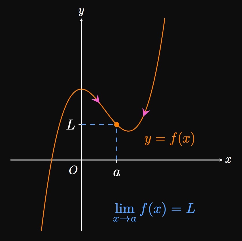
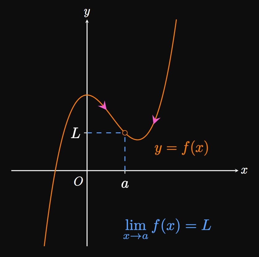
For example, in Figure 2A \(f(a)\) is defined
but in Figure 2B \(f(a)\) is undefined.
Yet in both cases, \(f(x)\) approaches \(L\) as \(x\) approaches \(a\)—meaning
both graphs satisfy \(\lim_{x \to a} f(x)\) \(= L.\)
| \(x\) | \(\ds f(x) = \frac{x^3 - 1}{x - 1}\) |
| \(0\) | \(1.0\) |
| \(0.2\) | \(1.24\) |
| \(0.6\) | \(1.96\) |
| \(0.9\) | \(2.71\) |
| \(0.99\) | \(2.9701\) |
| \(0.999\) | \(2.997\) |
| \(0.9999\) | \(2.9997\) |
| \(x\) | \(\ds f(x) = \frac{x^3 - 1}{x - 1}\) |
| \(1.0001\) | \(3.0003\) |
| \(1.001\) | \(3.003\) |
| \(1.01\) | \(3.0301\) |
| \(1.1\) | \(3.31\) |
| \(1.4\) | \(4.36\) |
| \(1.8\) | \(6.04\) |
| \(2\) | \(7.0\) |
| \(x\) | \(\ds f(x) = \frac{\sqrt{4 + x} - 2}{x}\) |
| \(-1\) | \(0.2679492\) |
| \(-0.8\) | \(0.263932\) |
| \(-0.4\) | \(0.2565835\) |
| \(-0.1\) | \(0.2515823\) |
| \(-0.01\) | \(0.2501564\) |
| \(-0.001\) | \(0.2500156\) |
| \(-0.0001\) | \(0.2500016\) |
| \(x\) | \(\ds f(x) = \frac{\sqrt{4 + x} - 2}{x}\) |
| \(0.0001\) | \(0.2499984\) |
| \(0.001\) | \(0.2499844\) |
| \(0.01\) | \(0.2498439\) |
| \(0.1\) | \(0.2484567\) |
| \(0.4\) | \(0.2440442\) |
| \(0.8\) | \(0.2386128\) |
| \(1\) | \(0.236068\) |
It's important to realize the limitations of using graphs and tables to estimate limits. Often, it's difficult to know how close to make \(x\) to \(a,\) and technology can mislead us. For example, in Example 2 if you make \(x\) small enough, then your calculator may return \(f(x) = 0.\) This result arises because for very small values of \(x,\) your calculator cannot hold enough digits to distinguish between \(\sqrt{4 + x}\) and \(2.\) Thus, the calculator returns the difference \(\par{\sqrt{4 + x} - 2}\) as \(0.\) But the limit \(\lim_{x \to 0} \par{\sqrt{4 + x} - 2}/x\) turns out to be \(1/4.\) In Section 1.2 we will discuss methods that permit us to calculate confidently, rather than guess, the values of such limits.
One-Sided Limits
One-sided limits are tools that extend our ability to describe functions. A left-hand limit gives the value to which \(f(x)\) tends as \(x\) is made close to \(a\) from strictly the left side; that is, we consider only \(x \lt a.\) We denote a left-hand limit using the notation \[\lim_{x \to a^-} f(x) = L \cma\] where the negative superscript on \(a^-\) suggests that \(x \lt a.\) (See Figure 3A.) Similarly, a right-hand limit is the value \(f(x)\) approaches as \(x\) is made close to \(a\) from solely the right side, so we consider only \(x \gt a.\) A right-hand limit is written as \[\lim_{x \to a^+} f(x) = L \cma\] for which the positive superscript on \(a^+\) implies that \(x \gt a.\) (See Figure 3B.) Note that we say \(x \lt a\) instead of \(x \leq a,\) and \(x \gt a\) instead of \(x \geq a.\)
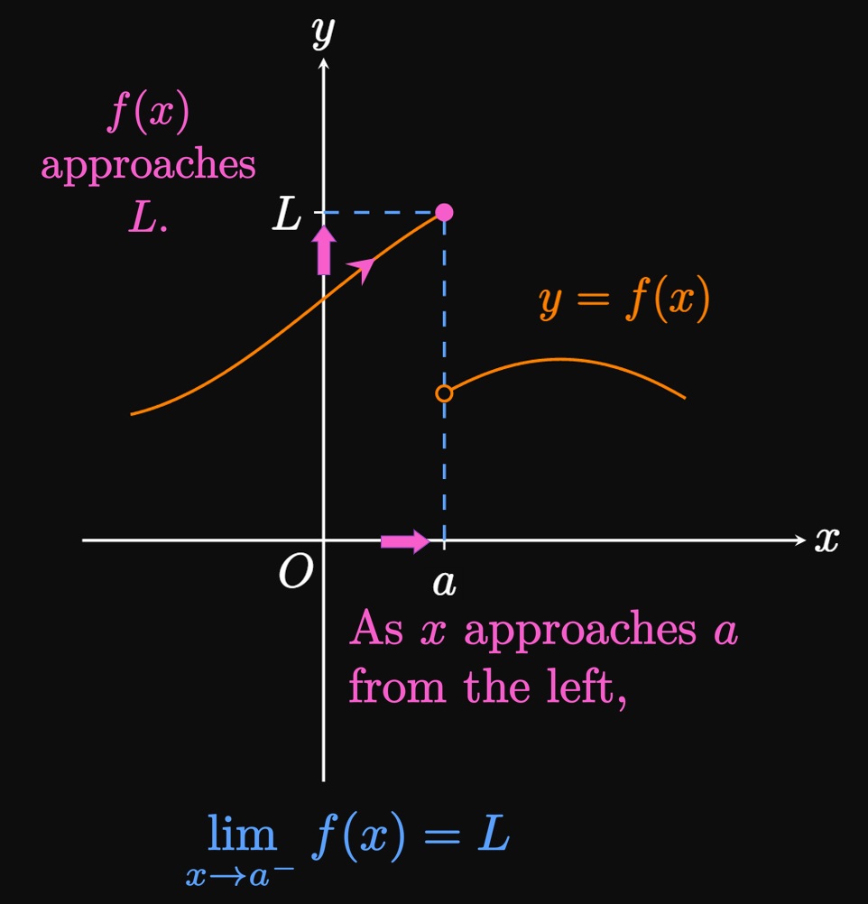
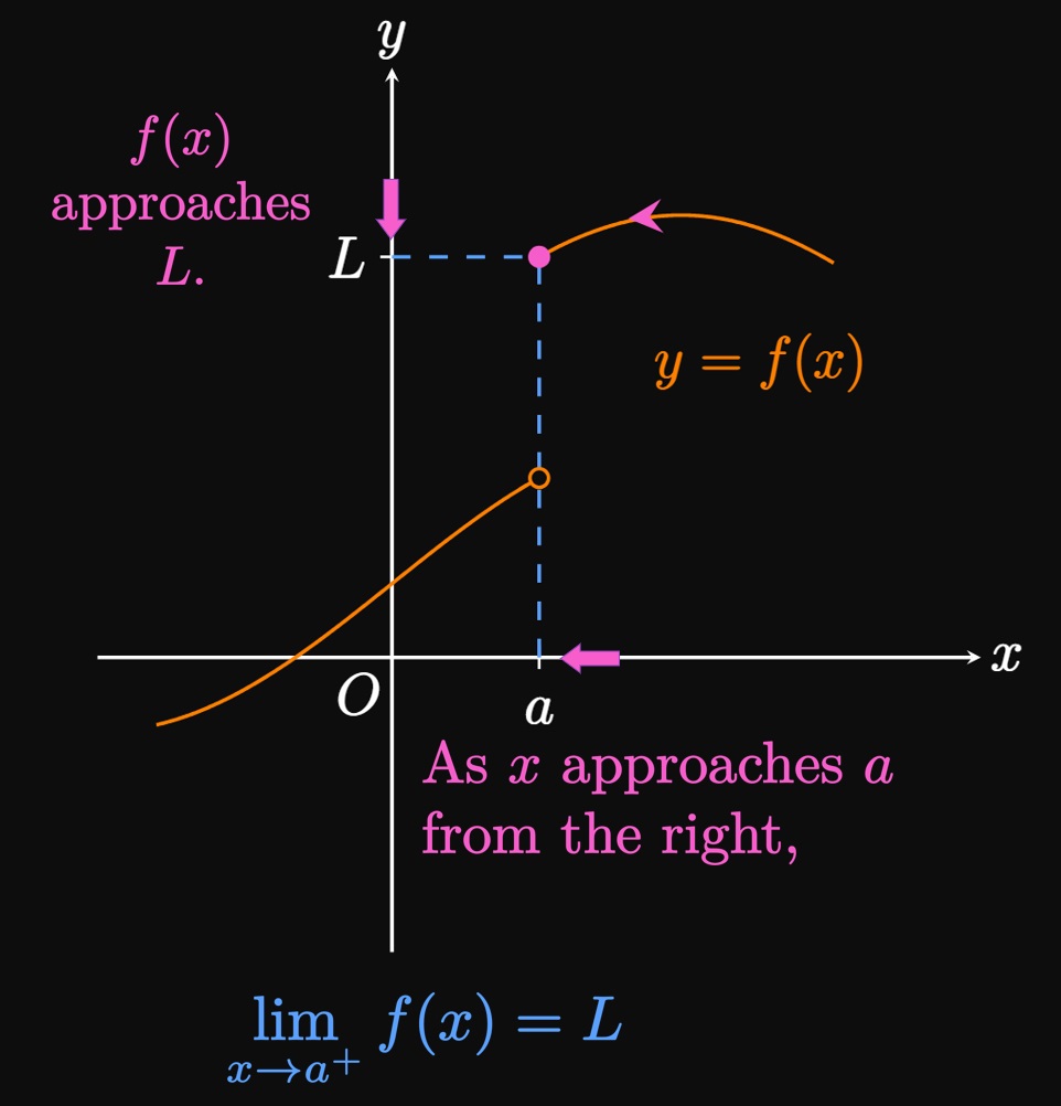
- Left-Hand Limits We write \[\lim_{x \to a^-} f(x) = L\] if \(f(x)\) can be made arbitrarily close to \(L\) as \(x\) is made sufficiently close to \(a\) (but not equal to \(a\)) for \(x\) less than \(a.\)
- Right-Hand Limits We write \[\lim_{x \to a^+} f(x) = L\] if \(f(x)\) can be made arbitrarily close to \(L\) as \(x\) is made sufficiently close to \(a\) (but not equal to \(a\)) for \(x\) greater than \(a.\)
Existence of a Limit A limit exists if and only if its one-sided limits exist and equal each other. Mathematically, \(\lim_{x \to a} f(x)\) \(= L\) is true if and only if \[\lim_{x \to a^-} f(x) = L \and \lim_{x \to a^+} f(x) = L \pd\] In other words, we must be able to trace a curve \(f\) near \(a\) and see the values of \(f(x)\) approach \(L\) from both sides of \(x = a.\) If this agreement isn't present, then the limit doesn't exist. For the graphs in Figure 3A and Figure 3B, the one-sided limits of \(f\) at \(a\) are different. Thus, for each graph \(\lim_{x \to a} f(x)\) does not exist.
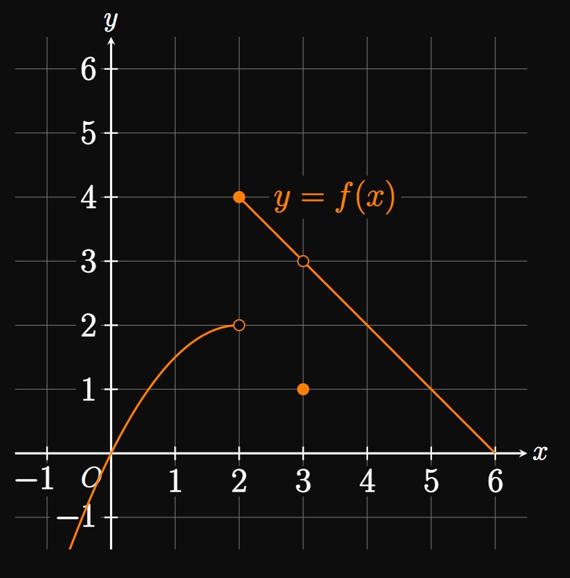
- \(\ds \lim_{x \to 0} f(x)\)
- \(\ds \lim_{x \to 2} f(x)\)
- \(\ds \lim_{x \to 3} f(x)\)
- Observe that \(f(x)\) approaches \(0\) as \(x\) is made close to \(0\) from both sides of \(0.\) So \[\lim_{x \to 0} f(x) = \boxed 0\]
- Tracing the graph from the left of \(x = 2,\) we see that \(f(x)\) approaches \(2.\) Conversely, as we trace the graph from the right of \(x = 2,\) we observe that \(f(x)\) approaches \(4.\) [In either case, we don't consider \(f(2)\).] We therefore write \[\lim_{x \to 2^-} f(x) = 2 \and \lim_{x \to 2^+} f(x) = 4 \pd\] Since these one-sided limits aren't equivalent, \(\lim_{x \to 2} f(x)\) does not exist.
- We see that \(f(x)\) approaches \(3\) as \(x\) approaches \(3\) from the left (that is, with \(x \lt 3\)). Similarly, \(f(x)\) tends to \(3\) as \(x\) is made close to \(3\) from the right (that is, for \(x \gt 3\)). Hence, \[\lim_{x \to 3^-} f(x) = \lim_{x \to 3^+} f(x) = 3 \pd\] Because both one-sided limits equal the same number \(3,\) we assert that \[\lim_{x \to 3} f(x) = \boxed 3\] Although \(f(3) = 1,\) the value of \(f\) at \(3\) has no relevance to the limit \(\lim_{x \to 3} f(x),\) which is the number \(f\) approaches as \(x \to 3.\)
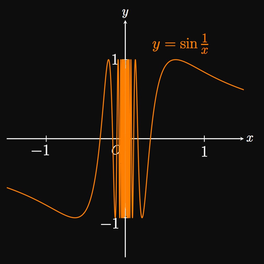
| \(x\) | \(\ds \frac{2}{\pi}\) | \(\ds \frac{2}{3\pi}\) | \(\ds \frac{2}{5\pi}\) | \(\ds \frac{2}{7\pi}\) | \(\ds \frac{2}{9\pi}\) | \(\ds \frac{2}{11\pi}\) |
| \(\ds \sin \frac{1}{x}\) | \(1\) | \(-1\) | \(1\) | \(-1\) | \(1\) | \(-1\) |
The preceding three examples show instances when a limit \(\lim_{x \to a} f(x)\) may fail to exist. A limit fails to exist if the one-sided limits of \(f\) at \(a\) don't agree with each other. Or a limit can fail to exist if \(f(x)\) doesn't settle to a final value—for example, \(f\) oscillates (such as in Example 5)—as \(x\) is made close to \(a.\)
Limits with Infinity
A function \(f(x)\) may approach some value \(L\) as \(x\) is made closer to some number \(a.\) But what if we let \(x\) increase or decrease without bound? In such cases, we aim to determine whether \(f(x)\) tends to a fixed number as \(x \to \infty\) or as \(x \to -\infty.\) We call these matters limits at infinity.
In general, the notation \[\lim_{x \to \infty} f(x) = L\] means that \(f(x)\) approaches some number \(L\) as we make \(x\) arbitrarily large (as large as we wish)—in other words, as \(x\) increases without bound. Similarly, writing \[\lim_{x \to -\infty} f(x) = L\] indicates that \(f(x)\) tends to \(L\) if we let \(x\) decrease without bound.
- If \(f(x)\) is defined for all \(x \geq a,\) then \[\lim_{x \to \infty} f(x) = L\] means that \(f(x)\) approaches \(L\) as \(x\) increases without bound.
- If \(f(x)\) is defined for all \(x \leq a,\) then \[\lim_{x \to -\infty} f(x) = L\] means that \(f(x)\) approaches \(L\) as \(x\) decreases without bound.
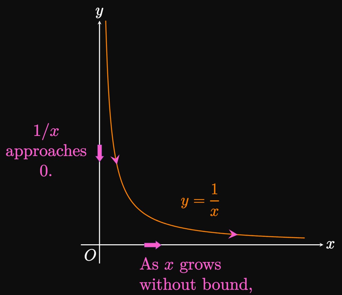
| \(x\) | \(\ds \frac{1}{x}\) |
| \(1\) | \(1\) |
| \(5\) | \(0.2\) |
| \(10\) | \(0.1\) |
| \(100\) | \(0.01\) |
| \(1000\) | \(0.001\) |
| \(10000\) | \(0.0001\) |
| \(100000\) | \(0.00001\) |
Infinite Limits
The notation
\[\lim_{x \to a} f(x) = \infty\]
means that the values of \(f(x)\) become bigger and bigger—increasing without bound—as \(x\) is made closer and closer to \(a.\)
We may choose to say a limit equals infinity
instead of writing does not exist,
which provides less information about a function's behavior.
The former statement concedes that a limit doesn't exist while communicating that the function
approaches \(\infty.\)
Likewise, writing
\[\lim_{x \to a} f(x) = -\infty\]
asserts that the values of \(f(x)\) decrease without bound as \(x\) approaches \(a.\)
This statement suggests that the limit fails to exist because \(f(x)\) approaches negative infinity.
In either definition, the value of \(f(a)\) (or whether it is undefined) is irrelevant.
- The statement \[\lim_{x \to a} f(x) = \infty\] means that \(f(x)\) increases without bound as \(x\) is made closer to \(a\) (but not equal to \(a\)).
- The statement \[\lim_{x \to a} f(x) = -\infty\] means that \(f(x)\) decreases without bound as \(x\) is made closer to \(a\) (but not equal to \(a\)).
Now let's merge the ideas of limits at infinity with infinite limits: The family of functions \(x^k,\) where \(k\) is a positive constant, satisfies \begin{equation} \lim_{x \to \infty} x^k = \infty \pd \label{eq:lim-x^k} \end{equation} This formula is intuitive because if \(x\) is large, then \(x^k\) is also large. Hence, \(x^k\) grows with \(x.\) Accordingly, the fraction \(1/x^k\) shrinks to \(0\) due to the division of \(1\) by an increasingly large number. Thus, \begin{equation} \lim_{x \to \infty} \frac{1}{x^k} = 0 \pd \label{eq:lim-1/x^k} \end{equation} In Example 6 we used this logic to verify \(\eqref{eq:lim-1/x^k}\) for \(k = 1.\)
CAUTION Understand that \(\infty\) is not a number. Saying a limit equals \(\infty\) or \(-\infty\) simply describes how the limit fails to exist, therefore providing us with more information about the function's behavior. We will elaborate on limits with infinity in Section 1.6.
- \(\ds \lim_{x \to \infty} \frac{1}{x^5}\)
- \(\ds \lim_{x \to \infty} \sqrt[3]{x}\)
- \(\ds \lim_{x \to \infty} x^{-2}\)
- We use \(\eqref{eq:lim-1/x^k},\) where \(k = 5 \gt 0,\) to assert that \[\lim_{x \to \infty} \frac{1}{x^5} = \boxed 0\]
- Rewriting \(\sqrt[3]{x}\) as \(x^{1/3},\) we apply \(\eqref{eq:lim-x^k}\) with \(k = 1/3 \gt 0\) to conclude \[\lim_{x \to \infty} \sqrt[3]{x} = \boxed{\infty}\] (We could also say the limit does not exist.)
- Since \(x^{-2} = 1/x^2,\) using \(\eqref{eq:lim-1/x^k}\) with \(k = 2 \gt 0\) shows \[\lim_{x \to \infty} x^{-2} = \lim_{x \to \infty} \frac{1}{x^2} = \boxed 0\]
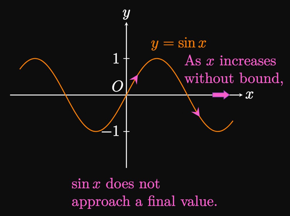
| \(x\) | \(\ds \frac{\pi}{2}\) | \(\ds \frac{3\pi}{2}\) | \(\ds \frac{5\pi}{2}\) | \(\ds \frac{7\pi}{2}\) | \(\ds \frac{9\pi}{2}\) | \(\ds \frac{11\pi}{2}\) |
| \(\ds \sin x\) | \(1\) | \(-1\) | \(1\) | \(-1\) | \(1\) | \(-1\) |
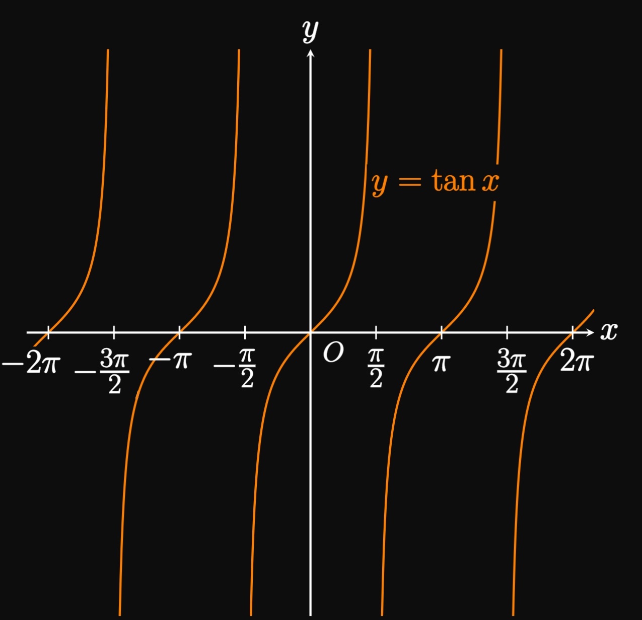
More generally, the limit as \(x \to \infty\) or \(x \to -\infty\) of any of the six trigonometric functions \((\sin x,\) \(\cos x,\) \(\tan x,\) \(\sec x,\) \(\csc x,\) and \(\cot x)\) does not exist. These graphs are periodic, meaning they constantly repeat themselves in regular intervals. Thus, none of these functions settles to a final value as \(x\) increases or decreases without bound.
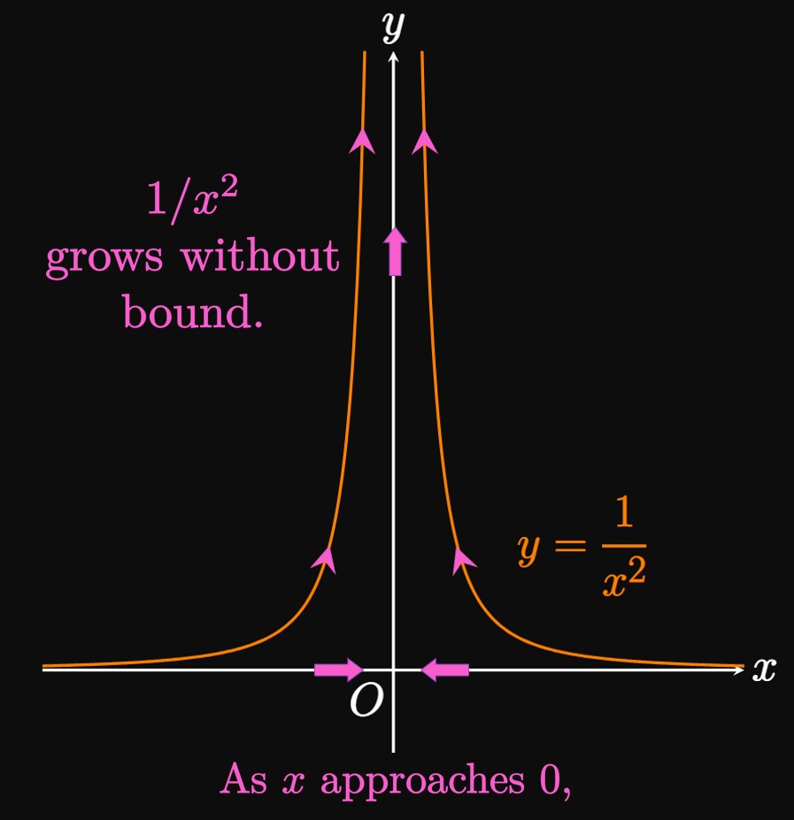
| \(x\) | \(\ds \frac{1}{x^2}\) |
| \(-1\) | \(1\) |
| \(-0.1\) | \(100\) |
| \(-0.01\) | \(10000\) |
| \(-0.001\) | \(1000000\) |
| \(-0.0001\) | \(100000000\) |
| \(x\) | \(\ds \frac{1}{x^2}\) |
| \(0.0001\) | \(100000000\) |
| \(0.001\) | \(1000000\) |
| \(0.01\) | \(10000\) |
| \(0.1\) | \(100\) |
| \(1\) | \(1\) |
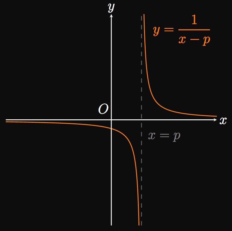
Example 9 shows that \(y = 1/x^2\) grows without bound as \(x\) is made closer to \(0.\) Specifically, \(y = 1/x^2\) has a vertical asymptote at \(x = 0\) because the curve becomes unbounded as \(x\) gets closer to \(0.\) Generally, a function \(f(x)\) has a vertical asymptote at \(x = p\) if any of the following is true: \[ \baat{2} \lim_{x \to p^-} f(x) &= \infty \lspace &&\lim_{x \to p^+} f(x) = \infty \nl \lim_{x \to p^-} f(x) &= -\infty \lspace &&\lim_{x \to p^+} f(x) = -\infty \pd \eaat \] In Figure 10, observe that the graph of \(y = 1/(x - p)\) has a vertical asymptote at \(x = p\) because \(\lim_{x \to p^-} f(x) = -\infty\) and \(\lim_{x \to p^+} f(x) = \infty.\)
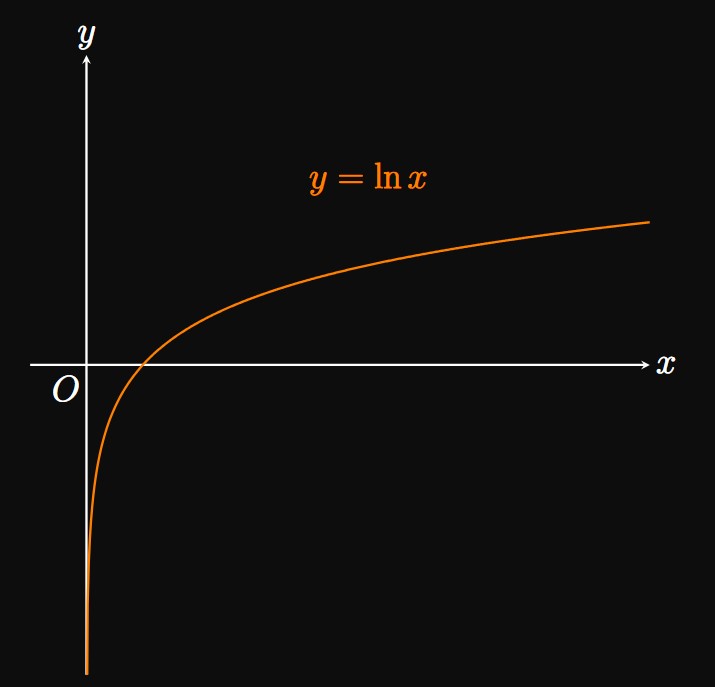
The graphs of many functions feature vertical asymptotes.
The natural logarithmic function \(y = \ln x,\)
for example, has a vertical asymptote at the \(y\)-axis (that is, at
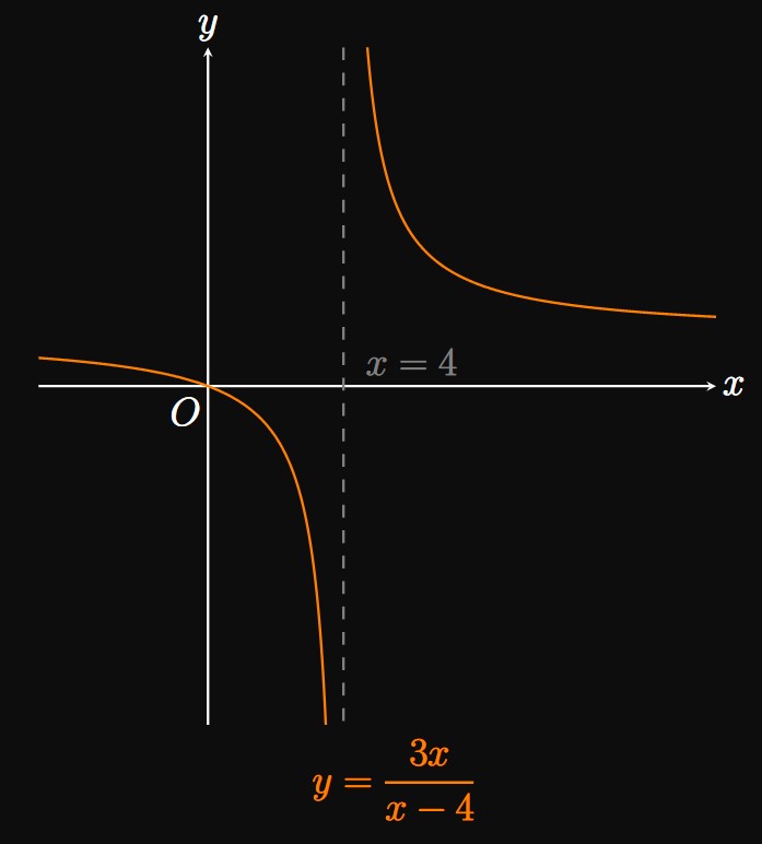
Left-Hand Limit If \(x\) is close to \(4\) but smaller than \(4,\) then the denominator \((x - 4)\) is a small negative number while the numerator \(3x\) remains positive. Accordingly, the fraction \(f(x) = 3x/(x - 4)\) is a large negative number. (A positive number is divided by a small negative number.) For example, \(f(3.9) = -117\) and \(f(3.99) = -1197.\) Thus, \(f(x)\) approaches \(-\infty\) as \(x \to 4^-,\) so we write \[\lim_{x \to 4^-} f(x) = \boxed{-\infty}\]
Right-Hand Limit For \(x\) close to \(4\) but bigger than \(4,\) the denominator \((x - 4)\) is a small positive number. At the same time, the numerator \(3x\) is positive. Hence, \(f(x) = 3x/(x - 4)\) is a large positive number. (A positive number is divided by a small positive number.) As an example, \(f(4.1) = 123\) and \(f(4.01) = 1203.\) The pattern is clear: As \(x \to 4^+,\) \(f(x)\) approaches \(\infty.\) So \[\lim_{x \to 4^+} f(x) = \boxed{\infty}\] (See Figure 13.)
Definition of a Limit (Intuitive)
A limit is the number \(f(x)\) approaches as
its input \(x\) approaches some number \(a.\)
We write
\[\lim_{x \to a} f(x) = L\]
if we can make the values of \(f(x)\) arbitrarily close to \(L\)
by making \(x\) sufficiently close to \(a\) on either side of \(a\)
but not equal to \(a.\)
We read this statement as follows: The limit, as \(x\) approaches \(a,\) of \(f(x)\) equals \(L.\)
In arrow notation, we write
\(f(x) \to L\) as \(x \to a.\)
Constructing a table with values of \(f\) close to \(a\)
can help us determine a limit, although tables and graphs can sometimes be misleading.
One-Sided Limits One-sided limits tell us what number \(f(x)\) approaches as \(x\) approaches \(a\) for either \(x \lt a\) or for \(x \gt a.\) Let \(f\) be defined near \(a\) (except possibly at \(a\) itself).
- Left-Hand Limits We write \[\lim_{x \to a^-} f(x) = L\] if \(f(x)\) can be made arbitrarily close to \(L\) as \(x\) is made sufficiently close to \(a\) (but not equal to \(a\)) for \(x\) less than \(a.\)
- Right-Hand Limits We write \[\lim_{x \to a^+} f(x) = L\] if \(f(x)\) can be made arbitrarily close to \(L\) as \(x\) is made sufficiently close to \(a\) (but not equal to \(a\)) for \(x\) greater than \(a.\)
If a function \(f(x)\) fails to settle to a single value as \(x \to a,\) then the limit \(\lim_{x \to a} f(x)\) does not exist. This can happen due to a disagreement in one-sided limits or if \(f\) oscillates as \(x \to a.\) The one-sided limits of a function \(f\) at \(a\) must be equivalent for \(\lim_{x \to a} f(x)\) to exist; namely, \(\lim_{x \to a} f(x) = L\) if and only if \[\lim_{x \to a^-} f(x) = L \and \lim_{x \to a^+} f(x) = L \pd\]
Limits with Infinity We can model the behavior of a function \(f(x)\) as \(x \to \infty\) or as \(x \to -\infty.\)
- If \(f(x)\) is defined for all \(x \geq a,\) then \[\lim_{x \to \infty} f(x) = L\] means that \(f(x)\) approaches \(L\) as \(x\) increases without bound.
- If \(f(x)\) is defined for all \(x \leq a,\) then \[\lim_{x \to -\infty} f(x) = L\] means that \(f(x)\) approaches \(L\) as \(x\) decreases without bound.
Let \(f\) be a function defined on both sides of \(a,\) except possibly at \(a\) itself.
- The statement \[\lim_{x \to a} f(x) = \infty\] means that \(f(x)\) increases without bound as \(x\) is made closer to \(a\) (but not equal to \(a\)).
- The statement \[\lim_{x \to a} f(x) = -\infty\] means that \(f(x)\) decreases without bound as \(x\) is made closer to \(a\) (but not equal to \(a\)).
Note that \(\infty\) is not a number. When we say a limit equals \(\infty\) or \(-\infty,\) we are implying that it does not exist while clarifying how it fails to exist. If \(k\) is a positive constant, then \begin{flalign} &&\lim_{x \to \infty} x^k &= \infty \eqlabel{eq:lim-x^k} &\nl \laWord{and} &&\lim_{x \to \infty} \frac{1}{x^k} &= 0 \pd \eqlabel{eq:lim-1/x^k} \end{flalign} The line \(x = p\) is a vertical asymptote of \(f(x)\) if any of the following is true: \[ \baat{2} \lim_{x \to p^-} f(x) &= \infty \lspace &&\lim_{x \to p^+} f(x) = \infty \nl \lim_{x \to p^-} f(x) &= -\infty \lspace &&\lim_{x \to p^+} f(x) = -\infty \pd \eaat \] Then the curve \(y = f(x)\) becomes unbounded on either side of the vertical asymptote. Algebraically, for rational functions, we identify locations of vertical asymptotes to be those such that the denominator is \(0\) while the numerator is nonzero.