7.2: Surface Areas of Revolution
A three-dimensional object has two properties of interest: volume (which we explored in Chapter 5) and surface area. We define a solid's surface area to be how much area its outer surface occupies. You are likely familiar with calculating surface areas of cubes and rectangular prisms, but how do we calculate the surface area of any smooth object? In this section we discuss how to find the surface area of the solid produced upon rotating a region about an axis.
Let's first establish formulas for the surface areas of simple solids.
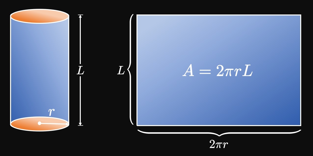
In Figure 1
the body of a cylinder of radius \(r\) and length \(L\) is unwrapped
into a rectangular sheet of dimensions \(L\) by \(2 \pi r\) (the circumference of the circular base).
The cylinder's lateral surface area is therefore \(A = 2 \pi r L.\)
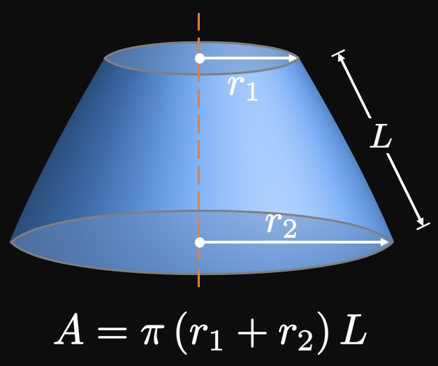
Conversely, to find the lateral surface area of a conical frustum
(a truncated right cone),
we average its radii \(r_1\) and \(r_2.\)
If \(L\) is the frustum's slant height,
then we treat it as a cylinder of length \(L\) and average radius \(r.\)
Since the average radius is \(r = \par{r_1 + r_2}/2,\)
the frustum's lateral surface area is
\begin{align}
A &= 2 \pi \par{\frac{r_1 + r_2}{2}} L \nonum \nl
&= \pi \par{r_1 + r_2} L \pd \label{eq:A-frus}
\end{align}
(See Figure 2.)
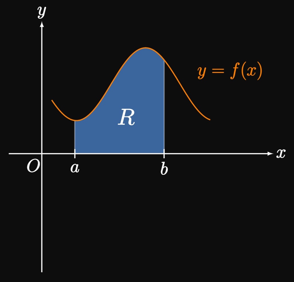
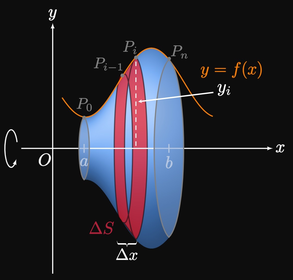
Surface Area of Smooth Solid Suppose that some region \(R,\) bounded by the smooth curve \(y = f(x)\) and the \(x\)-axis from \(x = a\) to \(x = b\) (Figure 3A), is rotated about the \(x\)-axis to generate a solid. We can calculate this solid's volume using the Disk and Washer Methods of Section 5.3. Yet to compute its lateral surface area, we employ a new strategy: We cut the interval \([a, b]\) into \(n\) subintervals with endpoints \(a = x_0, x_1,\) \(\dots, x_{n- 1},\) \(x_n = b\) and equal width \(\Delta x.\) In each subinterval we calculate the surface area of a band of the solid. Let \(P_0, P_1, \dots, P_n\) be points that lie on the curve. If \(n\) is small, then each approximating band resembles a conical frustum. Then we sum the surface areas of all \(n\) bands and take the limit as \(n \to \infty.\) In a general subinterval \(\parbr{x_{i - 1}, x_i},\) in which \(x_i^*\) is a sample point, the band's left radius is \(y_{i - 1},\) its right radius is \(y_i,\) and its slant height is \(\length{P_{i - 1} P_i}.\) (See Figure 3B.) By \(\eqref{eq:A-frus},\) the band's surface area is roughly \[\Delta S \approx 2 \pi \par{\frac{y_{i - 1} + y_i}{2}} \length{P_{i - 1} P_i} = \pi \par{y_{i - 1} + y_i} \length{P_{i - 1} P_i} \pd\] From Section 7.1, the arc length \(\length{P_{i - 1} P_i}\) is given by \(\sqrt{1 + [f'\par{x_i^*}]^2} \Delta x.\) Assuming \(\Delta x\) is small, and because \(f\) is continuous, we take \(y_{i - 1} = f \par{x_{i - 1}}\) \(\approx f \par{x_i^*}\) and \(y_i = f \par{x_i}\) \(\approx f \par{x_i^*}.\) Thus, we have \[\Delta S \approx \pi \parbr{2 f \par{x_i^*}} \sqrt{1 + [f'\par{x_i^*}]^2} \Delta x = 2 \pi f \par{x_i^*} \sqrt{1 + [f'\par{x_i^*}]^2} \Delta x \pd\] Summing the surface areas of all \(n\) bands, we obtain \[S = \lim_{n \to \infty} \sum_{i = 1}^n 2 \pi f \par{x_i^*} \sqrt{1 + [f'\par{x_i^*}]^2} \Delta x \pd\] As \(n \to \infty,\) our assumptions become more valid and the limit approaches the solid's surface area. We recognize the right-hand side as a Riemann sum for the function \(2 \pi f(x) \sqrt{1 + [f'(x)]^2},\) so we get \begin{equation} S = \int_a^b 2 \pi f(x) \sqrt{1 + [f'(x)]^2} \di x \pd \label{eq:A-x-f} \end{equation} Or in Leibniz notation, we write \[S = \int_a^b 2 \pi y \sqrt{1 + \par{\deriv{y}{x}}^2} \di x \pd\] Similarly, if a region is bounded between the smooth curve \(x = g(y)\) and the \(y\)-axis from \(y = c\) to \(y = d,\) then the surface area of the generated solid is \begin{equation} S = \int_c^d 2 \pi g(y) \sqrt{1 + [g'(y)]^2} \di y \cma \label{eq:A-y-g} \end{equation} or in Leibniz notation, \[S = \int_c^d 2 \pi x \sqrt{1 + \par{\deriv{x}{y}}^2} \di y \pd\]
General Formulas for Surface Area If we rotate a curve about the \(x\)-axis, then \(\eqref{eq:A-x-f}\) can only be used if we express all quantities in terms of \(x.\) Similarly, if we rotate about the \(y\)-axis, then \(\eqref{eq:A-y-g}\) is only applicable if we work entirely in terms of \(y.\) Yet sometimes we must rotate about an axis while using the opposite variable—for example, rotating about the \(x\)-axis while integrating with \(y.\) The following formulas provide us with this flexibility: We generalize \(\eqref{eq:A-x-f}\) as \begin{align} S &= \int_a^b 2 \pi y \di s \pd \label{eq:A-x} \end{align} Likewise, \(\eqref{eq:A-y-g}\) is generalized as \begin{align} S &= \int_c^d 2 \pi x \di s \pd \label{eq:A-y} \end{align} In each case, we choose the differential \(\dd s\) to be either \[\di s = \sqrt{1 + \par{\deriv{y}{x}}^2} \di x \or \di s = \sqrt{1 + \par{\deriv{x}{y}}^2} \di y \pd\]
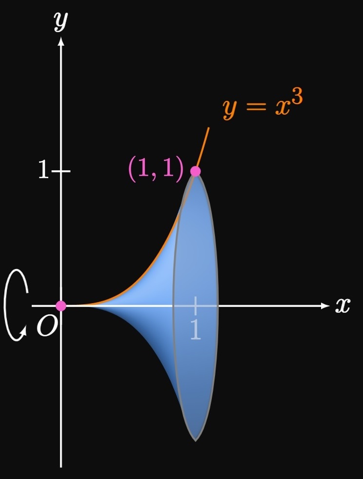
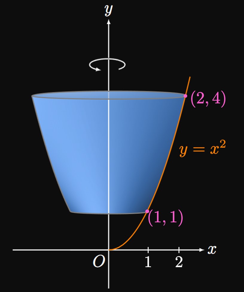
Method 1 (Integrating with
Method 2 (Integrating with
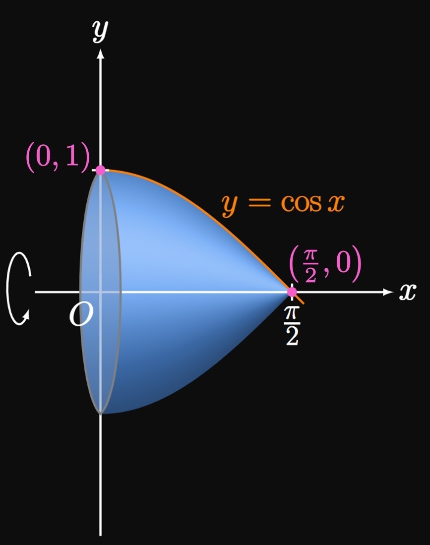
If the smooth curve \(y = f(x),\) \(a \leq x \leq b,\) is rotated about the \(x\)-axis, then the surface area of revolution is \begin{equation} S = \int_a^b 2 \pi f(x) \sqrt{1 + [f'(x)]^2} \di x \pd \eqlabel{eq:A-x-f} \end{equation} Likewise, if the smooth curve \(x = g(y),\) \(c \leq y \leq d,\) is rotated about the \(y\)-axis, then the surface area of revolution is \begin{equation} S = \int_c^d 2 \pi g(y) \sqrt{1 + [g'(y)]^2} \di y \pd \eqlabel{eq:A-y-g} \end{equation} More generally, we use the following formulas: \begin{alignat}{2} S &= \int_a^b 2 \pi y \di s \cma \lspace &&[\text{Rotating about } x \text{-Axis}] \eqlabel{eq:A-x} \nl S &= \int_c^d 2 \pi x \di s \cma \lspace &&[\text{Rotating about } y \text{-Axis}] \eqlabel{eq:A-y} \end{alignat} where \[\di s = \sqrt{1 + \par{\deriv{y}{x}}^2} \di x \or \di s = \sqrt{1 + \par{\deriv{x}{y}}^2} \di y \pd\]