4.3: Fundamental Theorem of Calculus

In Section 4.1 we discussed antiderivatives, and in Section 4.2 we introduced definite integrals to calculate areas. In this section, we connect both topics using the appropriately named Fundamental Theorem of Calculus, which links differential calculus to integral calculus. This section covers the following topics:

• Part I of the Fundamental Theorem of Calculus
• Using the Chain Rule in Part I of the Fundamental Theorem of Calculus
• Part II of the Fundamental Theorem of Calculus
• Net Change Theorem

Part I of the Fundamental Theorem of Calculus

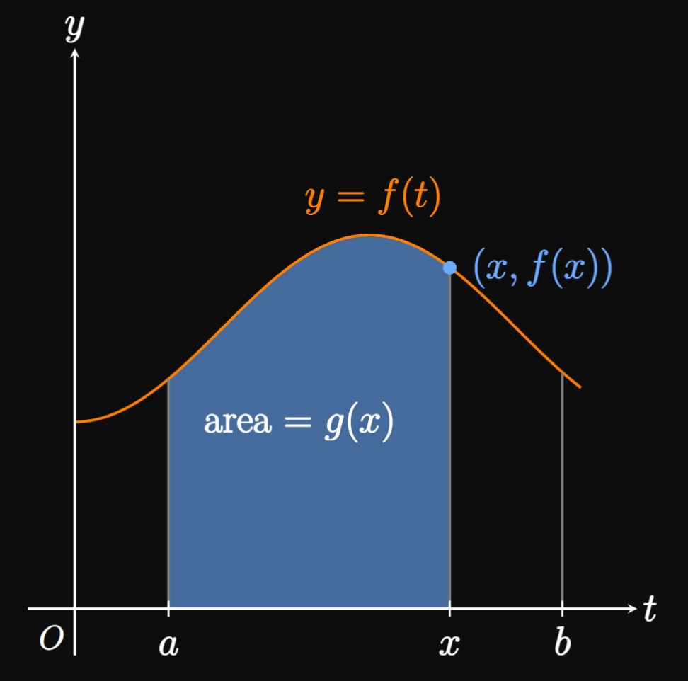
Let \(f(t)\) be a continuous function over the interval \(a \leq t \leq b,\) and let \begin{equation} g(x) = \int_a^x f(t) \di t \pd \label{eq:g} \end{equation} Note that \(x\) is a specific value of \(t\) and that \(g\) depends only on \(x.\) If \(f(t) \geq 0,\) then we interpret \(g\) as a function of area under the graph of \(y = f(t)\) from \(t = a\) to \(t = x.\) The area \(g(x)\) changes with \(x\) because adjusting \(x\) fluctuates the size of the region enclosed by \(f.\) (See Figure 1: Increasing \(x\) makes the region bigger, so \(g\) increases. Conversely, decreasing \(x\) shrinks the region, so \(g\) decreases.) If the enclosed region is below the \(t\)-axis, then the integral \(g(x) = \int_a^x f(t) \di t\) is a negative quantity. Note that if \(f\) is positive (as in Figure 1), then \(f(x)\) is the height of the curve above the \(t\)-axis when \(t = x.\) But if \(f\) is negative, then \(f(x)\) is the height of the curve under the \(t\)-axis.

Part I of the Fundamental Theorem of Calculus (which we abbreviate as FTC I) then asserts that \(g'(x) = f(x).\) If \(f(t) \geq 0,\) then FTC I asserts that the area \(g(x)\) is increasing at a rate equal to the height \(f(x).\) This interpretation is nearly the same if \(f(t) \leq 0 \col\) In this case, \(g\) is negative since the region enclosed by \(f\) is under the \(t\)-axis. So \(g\) is decreasing at a rate equal to the magnitude of the height \(f(x)\) below the \(t\)-axis. From another perspective, FTC I states that \(g\) is an antiderivative of \(f.\) (See Section 4.1 to review antiderivatives.) The theorem may be written equivalently in Leibniz notation as \begin{equation} \deriv{}{x} \int_a^x f(t) \di t = f(x) \pd \label{eq:ftc-I} \end{equation} In words, \(\eqref{eq:ftc-I}\) tells us that integrating a function \(f\) and then differentiating the result returns us the original function \(f.\) Thus, FTC I asserts that integration and differentiation are inverse operations—connecting rates of change to areas under curves. In \(\eqref{eq:ftc-I},\) we use \(t\) as a "dummy variable" because \(x\) is already used for the upper bound of the integral. Do not concern yourself with this distinction; the identity of \(f\) is the same regardless of whether we write \(f(t)\) or \(f(x).\)

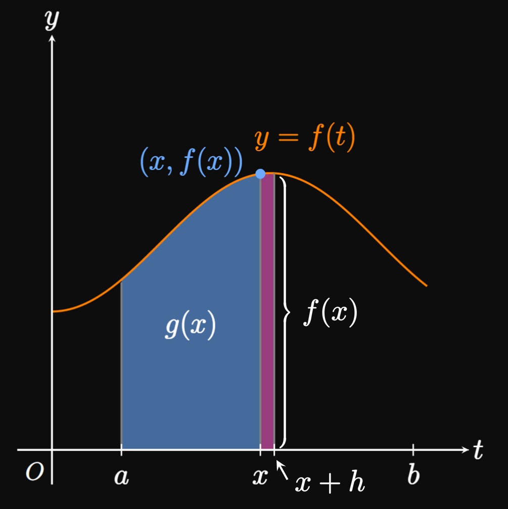
PROOF Let \(g(x) = \int_a^x f(t) \di t,\) and let \(h \gt 0\) be a small number. In Figure 2, the difference \(g(x + h) - g(x)\) is the pink region between \(t = x\) and \(t = x + h.\) We approximate this region as a rectangle of width \(h\) and height \(f(x) \col\) \[g(x + h) - g(x) \approx f(x) h \pd\] Solving for \(f(x)\) shows \[f(x) \approx \frac{g(x + h) - g(x)}{h} \pd\] As the width \(h\) becomes smaller, the region becomes closer to a rectangle, so the approximation increases in accuracy. Therefore, \[f(x) = \lim_{h \to 0} \frac{g(x + h) - g(x)}{h} \pd\] But the right-hand side is the limit definition of \(g'(x),\) so \(f(x) = g'(x).\) \[\qedproof\]

Using the Chain Rule in Part I of the Fundamental Theorem of Calculus

We now discuss definite integrals of \(f(t)\) in which the bounds are functions of \(x.\) In each case, assume \(f\) is continuous between the bounds.

Consider the derivative \(\textDeriv{}{x} \int_k^{u(x)} f(t) \di t,\) where \(k\) is a constant. We differentiate using the Chain Rule, treating the definite integral as a composite function in which \(u(x)\) is the inner function. In the integrand we replace \(t\) with \(u(x),\) but we then multiply by \(u'(x) \col\) \begin{equation} \deriv{}{x} \int_k^{u(x)} f(t) \di t = f(u(x)) \, u'(x) \pd \label{eq:ftc-chain-u} \end{equation} Now consider \(\textDeriv{}{x} \int_{v(x)}^k f(t) \di t.\) We rewrite the definite integral as \(-\int_k^{v(x)} f(t) \di t,\) and by analogy to \(\eqref{eq:ftc-chain-u}\) we have \begin{equation} \deriv{}{x} \int_{v(x)}^k f(t) \di t = -f(v(x)) \, v'(x) \pd \label{eq:ftc-chain-v} \end{equation} The most general case is \(\textDeriv{}{x} \int_{v(x)}^{u(x)} f(t) \di t.\) We split this integral at \(t = k,\) where \(v(x) \leq k \leq u(x).\) Therefore, \[ \ba \deriv{}{x} \int_{v(x)}^{u(x)} f(t) \di t &= \deriv{}{x} \parbr{\int_{v(x)}^k f(t) \di t + \int_k^{u(x)} f(t) \di t} \nl &= \deriv{}{x} \int_{v(x)}^k f(t) \di t + \deriv{}{x} \int_k^{u(x)} f(t) \di t \pd \ea \] Then, by \(\eqref{eq:ftc-chain-u}\) and \(\eqref{eq:ftc-chain-v},\) we have \begin{equation} \deriv{}{x} \int_{v(x)}^{u(x)} f(t) \di t = f(u(x)) \, u'(x) - f(v(x)) \, v'(x) \pd \label{eq:ftc-chain} \end{equation}

At first, \(\eqref{eq:ftc-chain}\) looks intimidating. This equation is difficult to memorize; instead, become familiar with the following procedure: First, replace \(t\) in the integrand with the upper function \(u(x)\) and multiply the result by \(u'(x).\) Then, replace \(t\) in the integrand with the lower function \(v(x)\) and multiply the result by \(v'(x).\) Finally, subtract the second term from the first term.

Part II of the Fundamental Theorem of Calculus

In Section 4.2, we calculated definite integrals using limits of Riemann sums. But what is the relationship between antidifferentiation and areas under curves? Part II of the Fundamental Theorem of Calculus (FTC II) relates the area under a graph to the difference in an antiderivative. If \(f\) is continuous over \([a, b]\) and \(F\) is an antiderivative of \(f,\) then \begin{equation} \int_a^b f(x) \di x = F(b) - F(a) \pd \label{eq:ftc-ii} \end{equation} Using \(\eqref{eq:ftc-ii}\) to calculate a definite integral is much easier than taking the limit of a Riemann sum. It is very remarkable that \(\int_a^b f(x) \di x\) is equivalent to the difference \(F(b) - F(a),\) which we may write as \(F(x) \Big|_a^b.\) The only limitation of \(\eqref{eq:ftc-ii}\) exists if it's difficult to determine an antiderivative of \(f.\) Hence, we sometimes define a function by a definite integral [such as in \(\eqref{eq:g}\)] if we cannot compute an antiderivative in terms of elementary functions (for example, polynomials, trigonometric functions, exponential functions, logarithmic functions).

PROOF Let \(g(x) = \int_a^x f(t) \di t,\) where \(f\) is continuous over \([a, b].\) Let \(F\) be an antiderivative of \(f.\) We know, from FTC I, that \(g'(x) = f(x)\) and so \(g\) is another antiderivative of \(f.\) Since antiderivatives all differ by a constant, we have \(g(x) = F(x) + C,\) where \(C\) is a constant. Note that \[g(a) = \int_a^a f(t) \di t = 0 \and g(b) = \int_a^b f(t) \di t \pd\] Thus, \begin{align} \int_a^b f(t) \di t &= g(b) - g(a) \label{eq:proof-ftc-2} \nl &= [F(b) + C] - [F(a) + C] \nonumber \nl &= F(b) - F(a) \nonumber \cma \end{align} where the constant term \(C\) cancels out. We can write the left-hand side of \(\eqref{eq:proof-ftc-2}\) as \(\int_a^b f(x) \di x\) to match the form of \(\eqref{eq:ftc-ii},\) the equation we have proved. \[\qedproof\]

The enclosed region is shown by Figure 3. The integral expression for this area is \[\int_0^{\pi/2} \cos x \di x \pd\] An antiderivative of \(\cos x\) is \(\sin x.\) Thus, \(\eqrefer{eq:ftc-ii}\) states that the integral is \[\sin x \intEval_0^{\pi/2} = \sin \tfrac{\pi}{2} - \sin 0 = \boxed 1\] This area is \(1.\)

When you first use FTC II, you're likely to commit sign errors. To rectify these mistakes, keep practicing. As you become familiar with the procedure of substituting the bounds, you'll begin to drop fewer negative signs and become more fluent with integration—the skill you need for the next sections of calculus.

Be careful not to write \(+ C\) when evaluating a definite integral. Only add this arbitrary constant when taking an indefinite integral.

Net Change Theorem

Consider \(f',\) the derivative of \(f.\) \(\eqrefer{eq:ftc-ii}\) can be written as \[\int_a^b f'(x) \di x = f(b) - f(a) \pd\] Adding \(f(a)\) to both sides gives \begin{equation} f(b) = f(a) + \int_a^b f'(x) \di x \pd \label{eq:net-change} \end{equation} \(\eqrefer{eq:net-change}\) is called the Net Change Theorem. It is very intuitive if we view \(f(a)\) as the initial quantity and \(f(b)\) as the final quantity. Then \(\int_a^b f'(x) \di x\) is the net change in \(f\)—the accumulation of its rate, \(f'.\)

In Section 4.1 we tackled particle motion problems by using antidifferentiation, substituting an initial condition, and solving for a constant of integration. But using the Net Change Theorem, as in Example 6, yields the same result, often through an easier process.