8.4: Logistic Models
In this section we introduce the logistic function, which has many applications in modeling population growth, disease spread, and social media engagement. We modify the exponential function (from Section 8.3) to characterize limited growth. This section covers the following topics:
Logistic Growth
In Section 8.3 we modeled populations that grow exponentially. Under these models, we assumed that species had the resources to reproduce indefinitely. Yet a limit exists to how many individuals a population can sustain; we call this limit the carrying capacity of an ecosystem. To model these ecosystems, we need a function that grows exponentially when the population is small but slows in growth as the population approaches its carrying capacity.
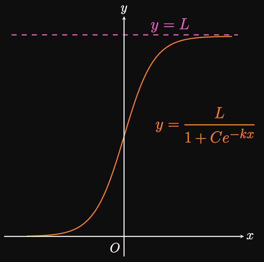
If \(y\) grows exponentially with \(x,\) then \(y\) satisfies the differential equation \[\deriv{y}{x} = ky \cma\] where \(k\) is a positive constant. To slow the growth as \(y\) approaches the carrying capacity \(L,\) we modify the exponential model by including the factor \(\par{1 - y/L}\) on the right side. Doing so gives the model \begin{equation} \deriv{y}{x} = ky \par{1 - \frac{y}{L}} \pd \label{eq:logistic-diff-eq} \end{equation} This differential equation defines logistic growth. Observe that as \(y\) grows toward \(L,\) the factor \((1 - y/L)\) approaches \(0\) and so \(\textDeriv{y}{x}\) approaches \(0.\) Accordingly, the growth of \(y\) is inhibited as \(y \to L.\) If \(y\) represents a population of animals and \(x\) is time, then the model in \(\eqref{eq:logistic-diff-eq}\) ensures the population growth slows toward \(0\) as the population approaches its carrying capacity. Note that the rate of change of \(y\) depends only on itself, not on \(x.\) The solution to \(\eqref{eq:logistic-diff-eq}\) is \begin{equation} y = \frac{L}{1 + Ce^{-kx}} \pd \label{eq:logistic-eq} \end{equation} We see that \[ \lim_{x \to \infty} \frac{L}{1 + Ce^{-kx}} = L \and \lim_{x \to -\infty} \frac{L}{1 + Ce^{-kx}} = 0 \pd \] Thus, \(y = 0\) and \(y = L\)—the line representing the carrying capacity—are horizontal asymptotes of a logistic model, assuming \(C \gt 0\) and \(k \gt 0.\) A quantity undergoing logistic growth is constantly increasing toward the carrying capacity. Because the graph's shape resembles the letter S, a logistic curve is sometimes called an S-curve. (See Figure 1.)
PROOF OF \(\eqref{eq:logistic-eq}\) We rewrite \(\eqref{eq:logistic-diff-eq}\) as \[ \ba \deriv{y}{x} &= ky \par{\frac{L - y}{L}} \nl \frac{1}{ky(L - y)} \di y &= \frac{1}{L} \di x \pd \nl \ea \] We break the left side into partial fractions (from Section 6.4): \begin{equation} \par{\frac{A}{ky} + \frac{B}{L - y}} \di y = \frac{1}{L} \di x \pd \label{eq:logistic-partial-fractions} \end{equation} On the left side, we see \[ \ba \frac{A}{ky} + \frac{B}{L - y} &= \frac{1}{ky(L - y)} \nl \frac{A(L - y) + Bky}{ky(L - y)} &= \frac{1}{ky(L - y)} \nl A(L - y) + Bky &= 1 \pd \ea \] Letting \(y = 0\) shows \[A(L - 0) + Bk(0) = 1 \implies A = \frac{1}{L} \pd\] Similarly, for \(y = L\) we see \[A(0) + Bk(L) = 1 \implies B = \frac{1}{kL} \pd\] Thus, \(\eqref{eq:logistic-partial-fractions}\) becomes \[ \ba \par{\frac{1/L}{ky} + \frac{1/kL}{L - y}} \di y &= \frac{1}{L} \di x \nl \par{\frac{1}{y} - \frac{1}{y - L}} \di y &= k \di x \pd \ea \] Integrating both sides gives \[ \ba \ln \abs{y} - \ln \abs{y - L} &= kx + C_1 \nl \ln \abs{y - L} - \ln \abs{y} &= C_1 - kx \nl \ln \abs{\frac{y - L}{y}} &= C_1 - kx \nl \ln \abs{1 - \frac{L}{y}} &= C_1 - kx \nl \ln \abs{\frac{L}{y} - 1} &= C_1 - kx \pd \ea \] We now exponentiate both sides, obtaining \[ \ba \abs{\frac{L}{y} - 1} &= e^{C_1 - kx} \nl &= e^{C_1} e^{-kx} \pd \ea \] If we let \(C = \pm e^{C_1},\) then we attain \begin{align} \frac{L}{y} &= 1 + Ce^{-kx} \nonum \nl \implies y &= \frac{L}{1 + Ce^{-kx}} \pd \eqlabel{eq:logistic-eq} \end{align} \[\qedproof\]
We compare this differential equation to \(\eqref{eq:logistic-diff-eq},\) where \(k = 0.05\) and \(L = 140.\) Thus, the general solution to the differential equation is, by comparison to \(\eqref{eq:logistic-eq},\) \[y = \frac{140}{1 + Ce^{-0.05x}}\] for some constant \(C.\)
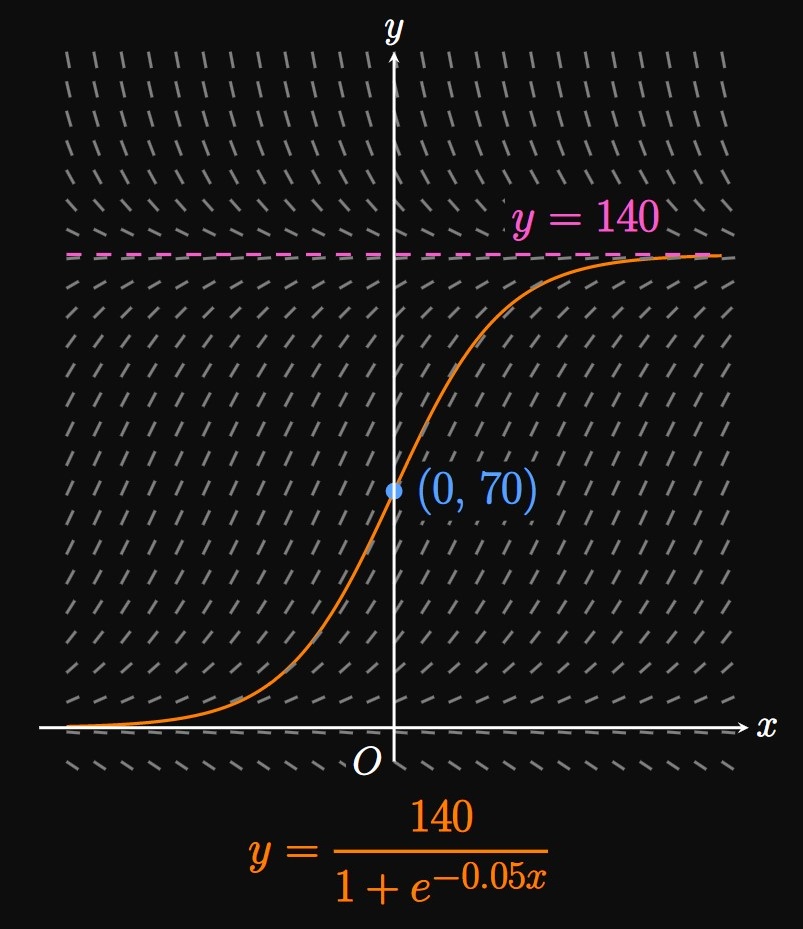
Solving for \(C\) We solve for \(C\) by substituting the initial condition \(y(0) = 70 \col\) \[ \ba \frac{140}{1 + Ce^{0}} &= 70 \nl 1 + C &= 2 \nl \implies C &= 1 \pd \ea \] Thus, the solution to this initial value problem is \[y = \boxed{\frac{140}{1 + e^{-0.05x}}}\] The solution curve passing through \((0, 70)\) is shown in Figure 2.
- Find the rate at which the population changes when there are \(50\) zebras.
- Determine the ecosystem's carrying capacity.
- What is the range of \(N(t)\) in context?
- When \(N = 50,\) we find the rate of change to be \[ \ba \deriv{N}{t} \intEval_{N = 50} &= 0.4 (50) \par{2 - \frac{50}{300}} \nl &= \tfrac{110}{3} \approx \boxed{36.667 \undiv{zebras}{yr}} \ea \]
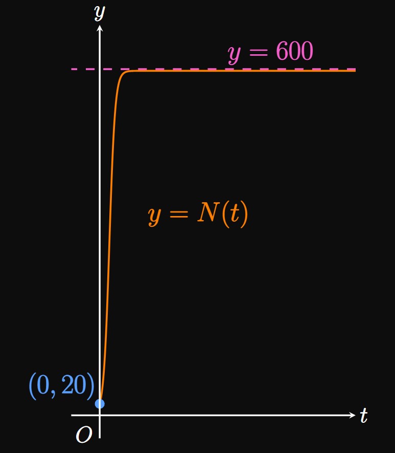
- Since a logistic curve flattens as the carrying capacity is reached, we let \(\textderiv{N}{t} = 0\) and solve for \(N.\) Doing so, we find \[ \ba 0.4N \par{2 - \frac{N}{300}} &= 0 \nl \implies N &= 0 \cma 600 \pd \ea \] We use the larger solution, so the carrying capacity is \(\boxed{600}\) zebras.
- Note that \(t \geq 0\) and \(N(0) = 20.\) Since \(N(t) \to 600\) as \(t \to \infty,\) the range is \(\boxed{[20, 600)}.\)
Because the population remains stable at \(1000,\) the carrying capacity of the ecosystem is \(L = 1000.\) Thus, \(\eqref{eq:logistic-eq}\) gives the model \[P(t) = \frac{1000}{1 + Ce^{-kt}} \cma\] where \(C\) and \(k\) are constants. Our strategy is to determine these constants by substituting the initial conditions \(P(0) = 50\) and \(P(3) = 200.\) Each initial condition allows us to solve for one constant; we therefore use two initial conditions to determine the two constants \(C\) and \(k.\)
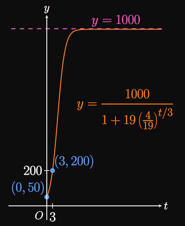
Solving for \(C\) and \(k\) Substituting \(P(0) = 50\) shows \[ \ba \frac{1000}{1 + Ce^{0}} &= 50 \nl 1 + C &= 20 \nl \implies C &= 19 \pd \ea \] Plugging in \(P(3) = 200\) reveals \[ \ba \frac{1000}{1 + 19e^{-3k}} &= 200 \nl 1 + 19e^{-3k} &= 5 \nl e^{-3k} &= \tfrac{4}{19} \nl \implies k &= -\tfrac{1}{3} \ln \tfrac{4}{19} \pd \ea \] Therefore, we have \[ \ba P(t) &= \frac{1000}{1 + 19e^{-\par{-\tfrac{1}{3} \ln \tfrac{4}{19}} t}} \nl &= \boxed{\frac{1000}{1 + 19 \par{\frac{4}{19}}^{t/3}}} \ea \] (See Figure 4.)
Logistic Decay
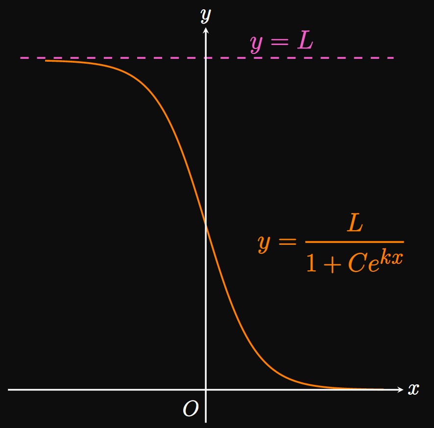
Whereas a quantity is increasing under logistic growth, a quantity is decreasing under logistic decay. Recall that \(y\) decays exponentially with \(x\) if \[\deriv{y}{x} = -ky \cma\] where \(k\) is a positive constant. Similar to our strategy in Logistic Growth, we tack on the factor \((1 - y/L)\) to attain \begin{equation} \deriv{y}{x} = -ky \par{1 - \frac{y}{L}} \pd \label{eq:decay-diff-eq} \end{equation} In this differential equation, the rate of decay of \(y\) slows as \(y\) approaches \(L.\) Because \(\eqref{eq:decay-diff-eq}\) is analogous to \(\eqref{eq:logistic-diff-eq}\) (the negative sign is the only discrepancy), its solution is given by replacing \(k\) with \(-k\) in \(\eqref{eq:logistic-eq} \col\) \begin{flalign} &&y &= \frac{L}{1 + Ce^{-(-k)x}} \nonum &\nl \laWord{or} && y &= \frac{L}{1 + Ce^{kx}} \pd \label{eq:logistic-decay} \end{flalign} For \(C \gt 0\) and \(k \gt 0,\) \[\lim_{x \to -\infty} \frac{L}{1 + Ce^{kx}} = L \and \lim_{x \to \infty} \frac{L}{1 + Ce^{kx}} = 0 \pd\] Thus, \(y = 0\) and \(y = L\) are the horizontal asymptotes of this curve. Unlike a logistic growth model, a logistic decay model approaches \(0\) as \(x \to \infty\) and is always decreasing on \(0 \lt y \lt L.\) (See Figure 5.)
Because \(\lim_{x \to -\infty} f(x) = 1500,\) the carrying capacity is \(L = 1500.\) \(\eqrefer{eq:logistic-decay}\) therefore gives the function \(f\) to be \[f(x) = \frac{1500}{1 + Ce^{kx}} \cma\] where \(C\) and \(k\) are constants. We determine their values by substituting the initial conditions \(f(0) = 700\) and \(f(5) = 400.\)
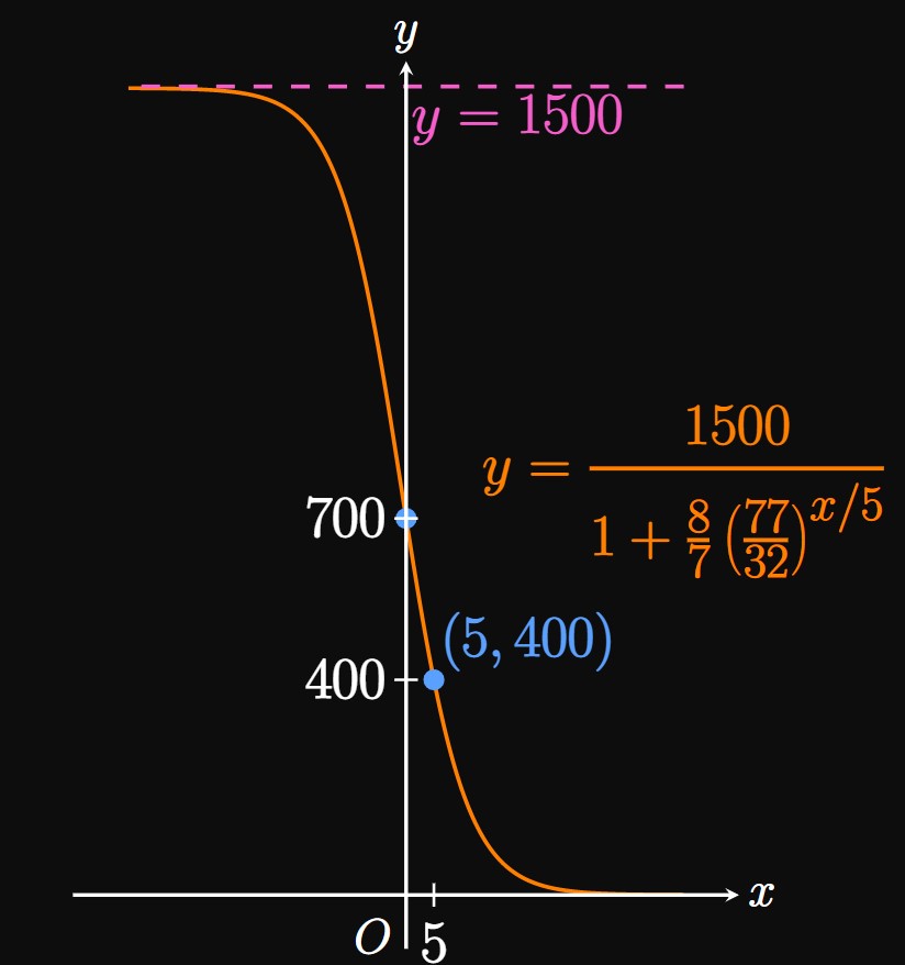
Solving for \(C\) and \(k\) Substituting \(f(0) = 700\) shows \[ \ba \frac{1500}{1 + Ce^0} &= 700 \nl 1 + C &= \tfrac{15}{7} \nl \implies C &= \tfrac{8}{7} \pd \ea \] Substituting \(f(5) = 400,\) we attain \[ \ba \frac{1500}{1 + \tfrac{8}{7}e^{5k}} &= 400 \nl 1 + \tfrac{8}{7}e^{5k} &= \tfrac{15}{4} \nl e^{5k} &= \tfrac{77}{32} \nl \implies k &= \tfrac{1}{5} \ln \tfrac{77}{32} \pd \ea \] Therefore, we have \[ \ba f(x) &= \frac{1500}{1 + \tfrac{8}{7} e^{\par{\tfrac{1}{5} \ln \tfrac{77}{32}}x}} \nl &= \boxed{\frac{1500}{1 + \tfrac{8}{7} \par{\tfrac{77}{32}}^{x/5}}} \ea \] (See Figure 6.)
Properties of Logistic Functions
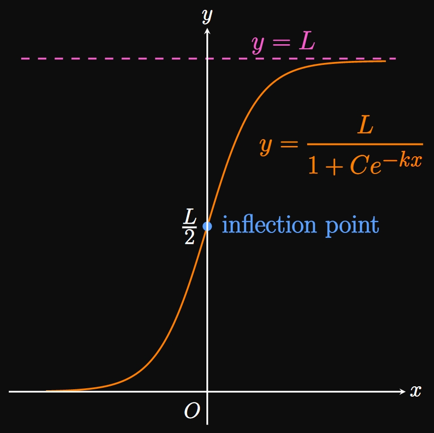
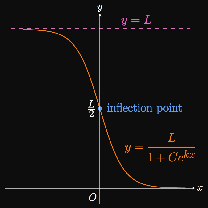
We can uncover many facts about a logistic function by determining its second derivative. In \(\eqref{eq:logistic-diff-eq}\) we use the Chain Rule to differentiate \(y\) with respect to \(x;\) doing so gives \[ \ba \derivOrder{y}{x}{2} &= k \deriv{y}{x} \par{1 - \frac{y}{L}} + ky \par{-\frac{1}{L}} \deriv{y}{x} \nl &= k \deriv{y}{x} \par{1 - \frac{2y}{L}} \pd \ea \] Recall, from Section 3.3, that a function has an inflection point when \(\textderivOrder{y}{x}{2}\) changes sign. We therefore equate the second derivative to \(0\) to see \[ \ba k \deriv{y}{x} \par{1 - \frac{2y}{L}} &= 0 \nl \implies y &= \frac{L}{2} \pd \ea \] Note that \(\textderiv{y}{x}\) never changes sign, and we attain the same result for logistic decay by differentiating \(\eqref{eq:decay-diff-eq}.\) At \(y = L/2,\) for both logistic growth and logistic decay, \(\textderivOrder{y}{x}{2}\) changes sign. Therefore, a logistic function has an inflection point when \(y\) reaches half of the carrying capacity. Also observe the following:
- The graph of a logistic function is concave up for \(y \lt L/2\) and concave down for \(y \gt L/2.\)
- A logistic growth function exhibits the fastest rate of growth when it reaches the inflection point at \(y = L/2.\) (See Figure 7A.)
- A logistic decay function decreases fastest upon reaching the inflection point at \(y = L/2.\) (See Figure 7B.)
| Condition | Logistic Growth, \(\ds \frac{L}{1 + Ce^{-kx}}\) | Logistic Decay, \(\ds \frac{L}{1 + Ce^{kx}}\) |
|---|---|---|
| As \(x \to \infty,\) | approaches \(L.\) | approaches \(0.\) |
| As \(x \to -\infty,\) | approaches \(0.\) | approaches \(L.\) |
| At \(y = L/2\) (inflection point), | increases most rapidly. | decreases most rapidly. |
| For \(y \lt L/2,\) | is concave up. | is concave up. |
| For \(y \gt L/2,\) | is concave down. | is concave down. |

Modeling Disease Logistic functions are excellent models for the recorded number of cases of a disease. One such example is modeling smallpox, a disease that ravaged the world for millennia. Fortunately, due to the advances in medicine and vaccine development, new cases became exceedingly rare in the 1950s and 1960s. In 1980, the World Health Organization declared smallpox to be eradicated; today, billions of children live without fear of smallpox. Figure 8 shows data points representing the number of total cumulative documented cases, in millions, of smallpox in the United States each year after 1900. By the method of regression analysis, the logistic growth function \[y = \frac{1.49}{1 + e^{-0.15(t - 1918)}}\] is a good fit for these data. Observe that the spread of smallpox accelerated from 1900 to 1920; around 1920, the logistic curve contains an inflection point—the point at which new cases were increasing most rapidly. But after hitting the inflection point, the spread of smallpox diminished between 1930 and 1940. (A logistic growth model is concave down for \(y\) past the inflection point, meaning the growth rate of \(y\) is decreasing.) In 1949 the last natural outbreak of smallpox occurred in the United States. Accordingly, our logistic model asserts that the total number of cases undergoes almost no change after \(t = 1949.\) Therefore, during an outbreak scientists often look for inflection points in the total number of recorded cases, since they signal diminishing infections ahead.
The disease's growth rate is highest when the number of total cases equals half of the carrying capacity, provided to be \(L = 2000.\) By \(\eqref{eq:logistic-eq}\) a logistic growth function for the number of cases is given by \[y = \frac{2000}{1 + Ce^{-kt}} \cma\] where \(t\) is time in days. We want to find the time \(t\) at which \(y = L/2\) \(= 1000.\)
Solving for \(C\) and \(k\) Note the initial conditions \(y(0) = 20\) and \(y(1) = 24.\) Substituting the former condition shows \[ \ba \frac{2000}{1 + Ce^{0}} &= 20 \nl 1 + C &= 100 \nl \implies C &= 99 \pd \ea \] Then substituting \(y(1) = 24\) reveals \[ \ba \frac{2000}{1 + 99e^{-k}} &= 24 \nl 1 + 99 e^{-k} &= \tfrac{250}{3} \nl \implies k &= -\ln \tfrac{247}{297} \pd \ea \] Thus, the logistic function modeling the cases of the virus is \[ \ba y &= \frac{2000}{1 + 99e^{-\par{-\ln \tfrac{247}{297}}t}} \nl &= \frac{2000}{1 + 99 \par{\tfrac{247}{297}}^t} \pd \ea \] We therefore see \[ \ba \frac{2000}{1 + 99 \par{\tfrac{247}{297}}^t} &= 1000 \nl 1 + 99 \par{\tfrac{247}{297}}^t &= 2 \nl \implies t &= \log_{247/297} \par{\tfrac{1}{99}} \approx \boxed{25 \un{days}} \ea \]
Logistic Growth The quantity \(y\) undergoes logistic growth with \(x\) if, for \(k \gt 0,\) \begin{equation} \deriv{y}{x} = ky \par{1 - \frac{y}{L}} \cma \eqlabel{eq:logistic-diff-eq} \end{equation} whose solution is \begin{equation} y = \frac{L}{1 + Ce^{-kx}} \pd \eqlabel{eq:logistic-eq} \end{equation} The quantity \(L\) is called the carrying capacity. In many applications, we take \(y\) to be population size and \(x\) to be time; then the carrying capacity can be interpreted as the maximum population size an ecosystem can sustain.
Logistic Decay The quantity \(y\) undergoes logistic decay with \(x\) if, for \(k \gt 0,\) \begin{equation} \deriv{y}{x} = -ky \par{1 - \frac{y}{L}} \cma \eqlabel{eq:decay-diff-eq} \end{equation} whose solution is \[ y = \frac{L}{1 + Ce^{kx}} \pd \eqlabel{eq:logistic-decay} \]
Properties of Logistic Functions The following table describes the properties of logistic growth functions and logistic decay functions, where \(C \gt 0\) and \(k \gt 0.\)
| Condition | Logistic Growth, \(\ds \frac{L}{1 + Ce^{-kx}}\) | Logistic Decay, \(\ds \frac{L}{1 + Ce^{kx}}\) |
|---|---|---|
| As \(x \to \infty,\) | approaches \(L.\) | approaches \(0.\) |
| As \(x \to -\infty,\) | approaches \(0.\) | approaches \(L.\) |
| At \(y = L/2\) (inflection point), | increases most rapidly. | decreases most rapidly. |
| For \(y \lt L/2,\) | is concave up. | is concave up. |
| For \(y \gt L/2,\) | is concave down. | is concave down. |