3.6: Optimization

To understand the problem, we experiment with some possibilities:

• If \(a = 13\) and \(b = 1,\) then their product is \(P = 13.\)
• If \(a = 12\) and \(b = 2,\) then their product is \(P = 24.\)
• If \(a = 11\) and \(b = 3,\) then their product is \(P = 33.\)

We want to find \(a\) and \(b\) that maximize the product \(P = ab\) and adhere to the condition \(a + b = 14.\) Since \(a\) and \(b\) add to \(14,\) \begin{equation} a + b = 14 \pd \label{eq:product-step-1} \end{equation} We want to maximize \begin{equation} P = ab \pd \label{eq:product-step-2} \end{equation} Our goal is to express \(P\) in terms of one variable—for example, \(a.\) From \(\eqref{eq:product-step-1},\) we find \(b = 14 - a.\) We substitute this expression into \(\eqref{eq:product-step-2}\) to get \[P = a(14 - a) = 14a - a^2 \pd\] We may now write \(P\) as \(P(a).\)

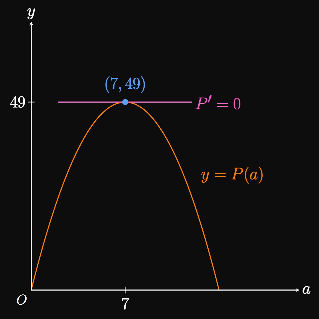
Optimization We find the critical numbers of \(P(a)\) by solving \(P'(a) = 0 \col\) \[ \ba P'(a) = 14 - 2a &= 0 \nl \implies a &= 7 \pd \ea \] For \(a \lt 7,\) \(P' \gt 0;\) for \(a \gt 7,\) \(P' \lt 0.\) Since \(P'(a)\) changes sign from positive to negative at \(a = 7,\) the First-Derivative Test states that \(a = 7\) is the location of a relative maximum of \(P.\) Also note the following:

• If \(a \lt 0,\) then \(b \gt 0\) and \(P \lt 0.\)
• If \(a \gt 14,\) then \(b \lt 0\) and \(P \lt 0.\)

Thus, \(a = 7\) must also correspond to the absolute maximum of \(P\) (see Figure 1). If \(a = 7,\) then \[b = 14 - 7 = 7\] and \(P = 7 \times 7 = 49.\) So \(\boxed{a = 7}\) and \(\boxed{b = 7}\) maximize the product \(P.\)

We create a sketch of the scenario (Figure 2). Let \(w\) denote the pen's width and \(\ell\) denote the pen's length. Also let \(A\) be the area of the pen. These suggestive variables help us avoid confusion. Let's construct a system of equations. The equation for the pen's perimeter is \begin{equation} 2w + \ell = 40 \pd \label{eq:farmer-1} \end{equation} We want to maximize \begin{equation} A = w \ell\ \pd \label{eq:farmer-2} \end{equation} Rearranging \(\eqref{eq:farmer-1}\) yields \(\ell = 40 - 2w,\) which we substitute into \(\eqref{eq:farmer-2}\) to acquire \[ A(w) = w \ell = w(40 - 2w) \pd\]

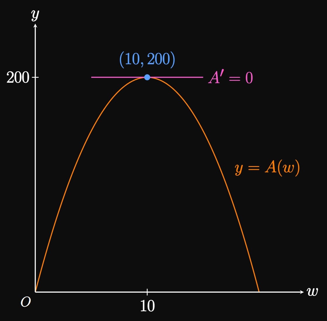
Optimization We differentiate \(A(w)\) and equate the result to \(0,\) seeing \[ \ba A'(w) = 40 - 4w &= 0 \nl \implies w &= 10 \pd \ea \] The domain in context is \(\{w \mid 0 \leq w \leq 20\};\) otherwise, side lengths become negative. The absolute maximum of \(A\) lies either at the endpoints of \(0 \leq w \leq 20\) or at its critical numbers. By the First-Derivative Test, \(w = 10\) corresponds to a relative maximum of \(A\) since \(A'(w)\) switches sign from positive to negative at \(w = 10.\) At \(w = 0\) and \(w = 20,\) \(A = 0\) because the pen collapses into a line. Thus, \(w = 10\) corresponds to the absolute maximum of \(A\) (Figure 3). For \(w = 10,\) we have \(\ell = 40 - 2(10) = 20.\) Thus, a pen of dimensions \(20\) feet by \(10\) feet produces the maximum area, \(200\) square feet.

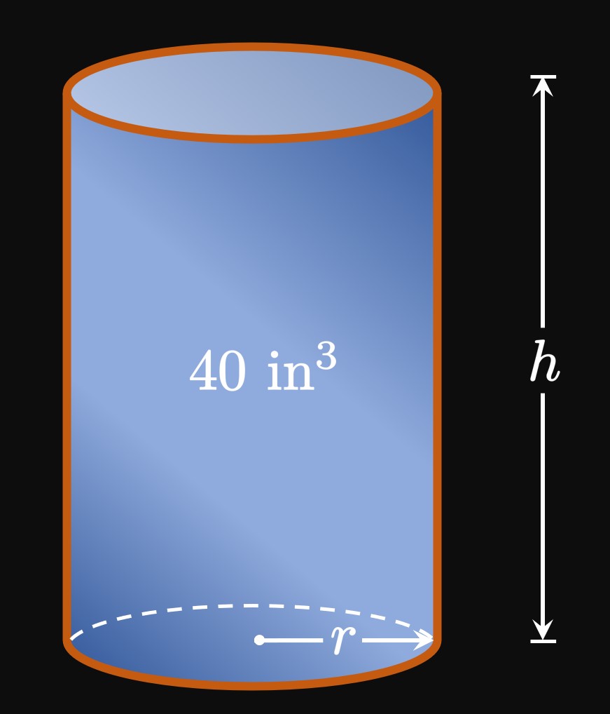
To understand the problem, we construct a picture (Figure 4). Let \(r\) be the can's radius and \(h\) be its height. The volume of the cylinder is then \begin{equation} 40 = \pi r^2 h \pd \label{eq:equation-cylinder-volume} \end{equation} We want to minimize the surface area: \begin{equation} S = 2 \pi r^2 + 2 \pi r h \pd \label{eq:equation-cylinder-SA} \end{equation} (To remember this formula, see that the bases of the can are circles of area \(\pi r^2,\) and a rectangular sheet of area \(2 \pi r h\) is wrapped around the can.) We aim to express \(S\) in terms of one variable. From \(\eqref{eq:equation-cylinder-volume},\) we have \(h = 40/(\pi r^2),\) which we substitute into \(\eqref{eq:equation-cylinder-SA}\) to get \[ \ba S(r) &= 2 \pi r^2 + 2 \pi r \left(\frac{40}{\pi r^2}\right) \nl &= 2 \pi r^2 + \frac{80}{r} \pd \ea \]

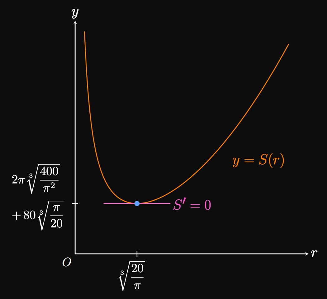
Optimization Differentiating \(S(r)\) gives \[S'(r) = 4 \pi r - \frac{80}{r^2} \pd\] To determine the critical numbers, we solve \(S'(r) = 0,\) as follows: \[ \ba S'(r) = 4 \pi r - \frac{80}{r^2} &= 0 \nl \implies r &= \sqrt[3]{\frac{20}{\pi}} \pd \nl \ea \] For \(r \lt \sqrt[3]{20/\pi},\) \(S' \lt 0;\) for \(r \gt \sqrt[3]{20/\pi},\) \(S' \gt 0.\) Since \(S'\) changes sign from negative to positive at \(r = \sqrt[3]{20/\pi},\) this value corresponds to a relative minimum of \(S\) by the First-Derivative Test. Also, because \(\lim_{r \to 0^+} S(r) = \infty\) and \(\lim_{r \to \infty} S(r) = \infty,\) there needs to be a minimum value of \(S(r),\) which must exist at the critical number (Figure 5). So \(r = \sqrt[3]{20/\pi}\) corresponds to the absolute minimum of \(S.\) We then have \(r \approx 1.853 \un{in}\) and \[h = \frac{40}{\pi (20/\pi)^{2/3}} \approx 3.707 \un{in} \pd\] Thus, a can of radius \(1.853 \un{in}\) and height \(3.707 \un{in}\) minimizes the materials used while holding the required volume. With a radius of \(1.853 \un{in},\) the cylinder's diameter is \(3.707 \un{in}\)—the same dimension as the height. The minimized surface area is \[ \ba S \par{\sqrt[3]{\frac{20}{\pi}}} &= 2 \pi \par{\sqrt[3]{\frac{20}{\pi}}}^2 + \frac{80}{\sqrt[3]{20/\pi}} \nl &= 2 \pi \sqrt[3]{\frac{400}{\pi^2}} + 80 \sqrt[3]{\frac{\pi}{20}} \nl &\approx 64.747 \un{in}^2 \pd \ea \]

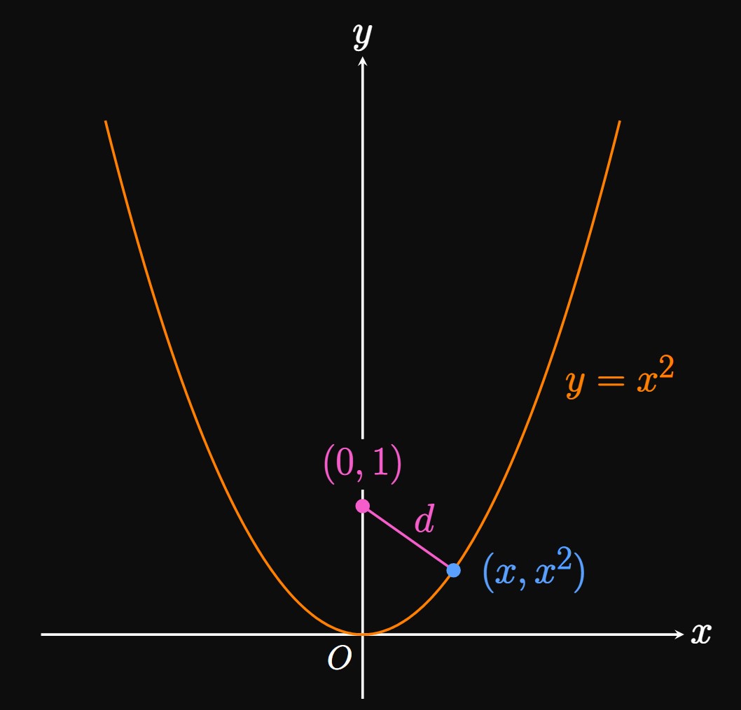
Figure 6 shows a sketch of the parabola and the points \((0, 1)\) and \((x, y)\) \(= (x, x^2).\) The distance between the points is, by the Distance Formula, \[ \ba d &= \sqrt{(x - 0)^2 + (y - 1)^2} \nl &= \sqrt{(x - 0)^2 + (x^2 - 1)^2} \nl &= \sqrt{x^4 - x^2 + 1} \pd \ea \]

Optimization We need to find the critical numbers of \(d.\) But \(d^2\) has the same critical numbers, so we choose to optimize \(d^2\) for convenience: Let \(q(x) = d^2\) \(= x^4 - x^2 + 1,\) whose derivative is \[q'(x) = 4x^3 - 2x \pd\] Solving \(q'(x) = 0,\) we find \[ \ba 4x^3 - 2x &= 0 \nl 2x(2x^2 - 1) &= 0 \nl \implies x &= 0 \cma \frac{-1}{\sqrt 2} \cma \frac{1}{\sqrt 2} \pd \ea \]

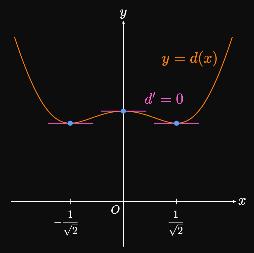
Note that \(q'\) changes sign from positive to negative at \(x = 0,\) so this value corresponds to a relative maximum of \(q\) by the First-Derivative Test. But we seek to minimize \(q,\) so we ignore this critical number. Conversely, \(q'\) changes sign from negative to positive at both \(x = -1/\sqrt 2\) and \(x = 1/\sqrt 2.\) So both values are locations of relative minima of \(q.\) Because \[\lim_{x \to -\infty} q(x) = \infty \and \lim_{x \to \infty} q(x) = \infty \cma\] the absolute minima of \(q\)—and therefore the absolute minima of \(d\)—must occur when \(x = -1/\sqrt 2\) and \(x = 1/\sqrt 2\) (Figure 7). At each value, \(y = (\pm 1/\sqrt 2)^2\) \(= 1/2.\) Thus, the closest points on the parabola to \((0, 1)\) are \[\boxed{\par{\frac{-1}{\sqrt 2} \cma \frac{1}{2}}} \and \boxed{\par{\frac{1}{\sqrt 2} \cma \frac{1}{2}}}\] as we expect from the parabola's symmetry.

REMARK If we differentiated \(d,\) then we would've gotten \[d'(x) = \frac{4x^3 - 2x}{\sqrt{x^4 - x^2 + 1}} \cma\] which has the same zeros as \(q'(x),\) confirming that \(d\) and \(q(x) = d^2\) have the same critical numbers.

The word inscribed means the rectangle has two vertices on the parabola and two vertices on the \(x\)-axis (Figure 8). Since the rectangle has length \(2x\) and height \(y,\) its area is \begin{equation} A = 2xy \pd \label{eq:inscribe-area} \end{equation} But \(y = 9 - x^2,\) so \(\eqref{eq:inscribe-area}\) becomes \[A(x) = 2x(9 - x^2) \pd\] We solve \(A'(x) = 0,\) finding \[ \ba A'(x) = 18 - 6x^2 &= 0 \nl \implies x &= -\sqrt 3 \cma \sqrt 3 \pd \ea \] The domain of \(A(x)\) in context is \(\{x \mid 0 \leq x \leq 3\},\) so we discard \(x = - \sqrt 3.\) The value \(x = \sqrt 3\) corresponds to a relative maximum of \(A\) because \(A'\) changes sign from positive to negative at that point. At each endpoint, \(A = 0\) since the rectangle collapses into a line. Thus, \(x = \sqrt 3\) is the location of the absolute maximum of \(A.\) Then \(y = 9 - (\sqrt 3)^2 = 6,\) so \(\eqref{eq:inscribe-area}\) gives the maximum area to be \[A = 2(\sqrt 3)(6) = \boxed{12 \sqrt 3}\]

We seek an expression for the time, \(t,\) the lifeguard takes to rescue the swimming person. The distance she runs is \(x,\) and the distance she swims is (by the Distance Formula) \(\sqrt{(20 - x)^2 + 64}.\) Note that \(\text{time}\) \(= \text{distance}/\text{speed}.\) The lifeguard's speed is \(10\) feet per second onshore and \(6\) feet per second in water. Therefore, her time for the first part of the trip, running onshore, is \[t_1 = \frac{x}{10} \pd\] Her time for the second part of the trip, swimming, is \[t_2 = \frac{\sqrt{(20 - x)^2 + 64}}{6} \pd\] The total time, \(t,\) is the sum of these times: \[ \ba t &= t_1 + t_2 \nl &= \frac{x}{10} + \frac{\sqrt{(20 - x)^2 + 64}}{6} \nl &= \frac{x}{10} + \frac{\sqrt{x^2 - 40x + 464}}{6} \pd \ea \]

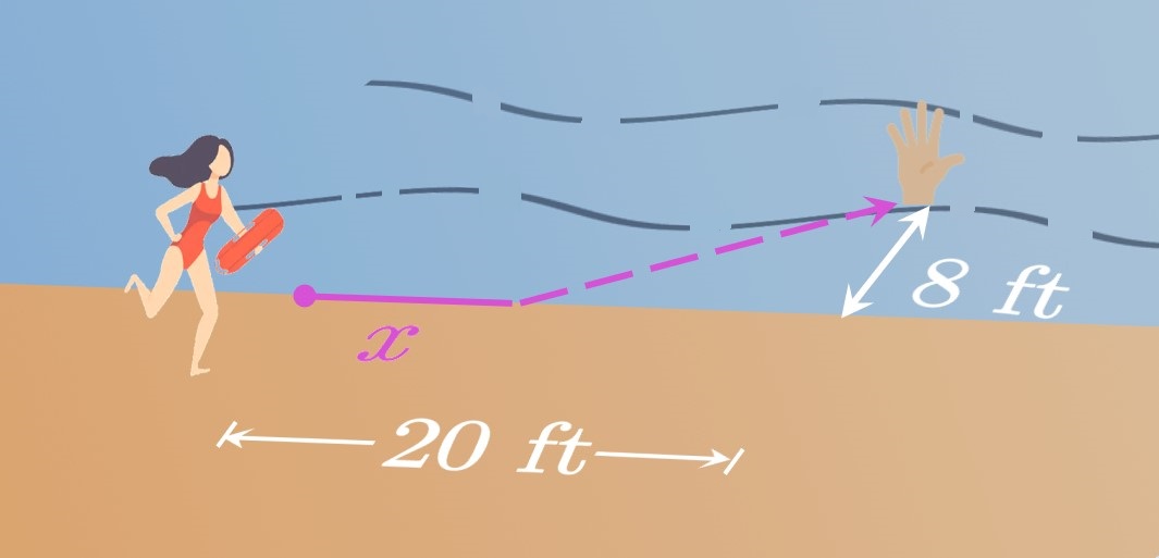
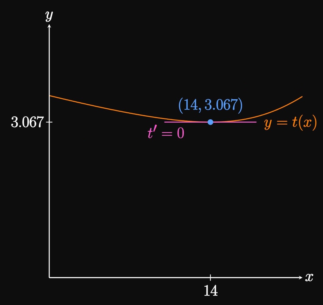
Optimization Differentiating with respect to \(x\) shows \[ t'(x) = \frac{1}{10} + \frac{x - 20}{6 \sqrt{x^2 - 40x + 464}} \pd \] To locate the critical numbers of \(t,\) we solve \(t'(x) = 0,\) as follows: \[ \ba \frac{1}{10} + \frac{x - 20}{6 \sqrt{x^2 - 40x + 464}} &= 0 \nl \frac{6 \sqrt{x^2 - 40x + 464} + 10 x - 200}{60 \sqrt{x^2 - 40x + 464}} &= 0 \nl 6 \sqrt{x^2 - 40x + 464} + 10 x - 200 &= 0 \nl 6 \sqrt{x^2 - 40x + 464} &= -10x + 200 \nl 36 \par{x^2 - 40x + 464} &= 100x^2 - 4000x + 40000 \nl 64 (x - 26)(x - 14) &= 0 \nl \implies x &= 14 \cma 26 \pd \ea \] The domain of \(t(x)\) in context is \(\{x \mid 0 \leq x \leq 20\},\) so the solution \(x = 26\) is extraneous. Observe that \(t' \lt 0\) for \(0 \leq x \lt 14\) and \(t' \gt 0\) for \(14 \lt x \leq 20.\) Hence, \(t\) has a relative minimum at \(x = 14\) by the First-Derivative Test. Note that \(t(0) \approx 3.590,\) \(t(14) \approx 3.067,\) and \(t(20) \approx 3.333.\) Consequently, \(t\) has an absolute minimum at \(x = 14\) (Figure 10). So the lifeguard should run \(\boxed{14 \un{ft}}\) before jumping in the water to save the swimmer in just \(3.067\) seconds.

The three angles \[\andThree{\theta}{\tan^{-1} \par{\frac{x}{4}}}{\tan^{-1} \par{\frac{3}{x + 1}}}\] must add to \(\pi.\) Thus, we have \[\theta = \pi - \tan^{-1} \left( \frac{x}{4} \right) - \tan^{-1} \left(\frac{3}{x + 1}\right) \pd\] To avoid any negative side lengths, the domain in context is \(0 \lt x \lt \infty.\) Graphing the function \(y = \theta(x)\) on \((0, \infty)\) reveals the absolute maximum of \(\theta\) to occur when \(\boxed{x = 0.899}.\)

Let \(x\) be the distance from the anchor point to the left tower's base. Then the distance from the anchor point to the right tower's base is \((30 - x).\) The wire needed to connect the anchor point to the top of the left tower is, by the Distance Formula, \[w_1 = \sqrt{x^2 + 10^2} = \sqrt{x^2 + 100} \pd\] Likewise, the wire needed to connect the anchor point to the top of the right tower is \[w_2 = \sqrt{(30 - x)^2 + 15^2} = \sqrt{x^2 - 60x + 1125} \pd\] Therefore, the total required amount of wire is \[ \ba w &= w_1 + w_2 \nl &= \sqrt{x^2 + 100} + \sqrt{x^2 - 60x + 1125} \pd \ea \]

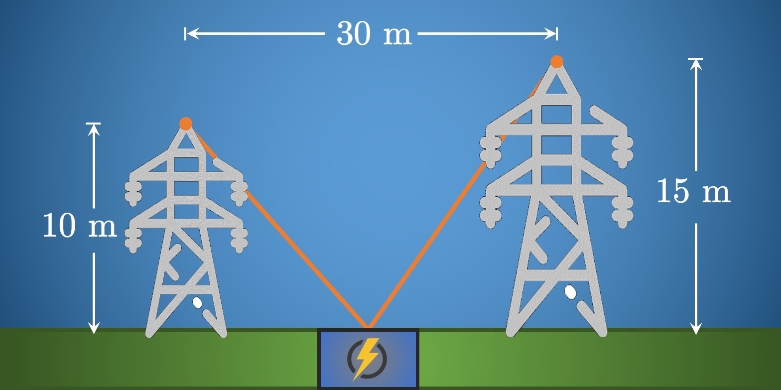
Optimization Differentiating \(w\) to locate its critical points, we see \[ \ba \frac{\dd w}{\dd x} = \frac{x}{\sqrt{x^2 + 100}} + \frac{x - 30}{\sqrt{x^2 - 60x + 1125}} &= 0 \nl \implies x &= 12 \pd \ea \] By graphing \(y = w(x),\) you may convince yourself that this critical number is the location of the absolute minimum of \(w.\) Thus, the optimal spot to anchor the wires is \(\boxed{12 \un{m}}\) to the right of the left tower.