4.2: Definite Integrals
One of the key goals of calculus is to determine the area of any shape. It is easy to calculate areas of simple geometric figures such as rectangles, squares, and even hexagons. But for other shapes, especially if their edges are curved and they are asymmetrical, we need a new strategy since no simple geometric formula exists for the area. Areas under curves enable us to calculate many quantities, such as displacement from velocity, change in volume from flow rate, and energy from power. These concepts are linked to the integral, which forms the entire basis of integral calculus—the second big half of calculus, following differential calculus. We discuss the following topics:
- Areas under Curves
- Defining a Definite Integral
- Evaluating Definite Integrals
- Properties of Definite Integrals
- Comparison Properties of Definite Integrals
Areas under Curves
In Figure 1A, consider the region \(R\) bounded between the continuous curve \(y = f(x)\) and the \(x\)-axis from \(x = a\) to \(x = b.\)

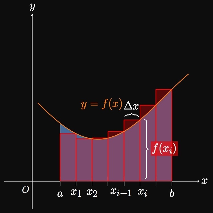

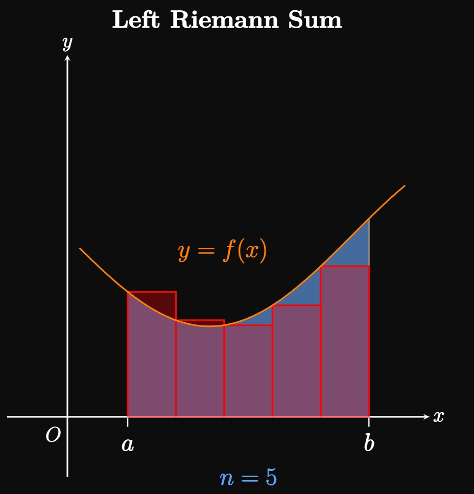
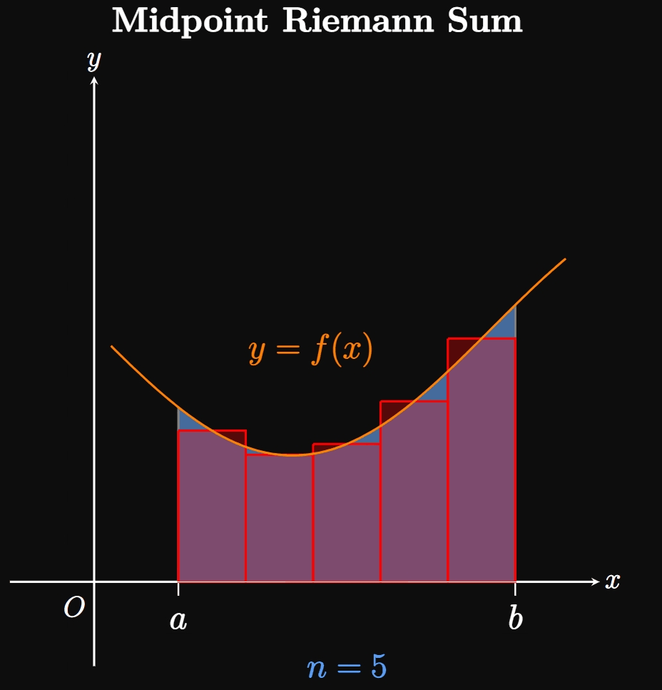
We can estimate the area of \(R\) by inscribing a number \(n\) of rectangles under the curve. In Figure 1B, we split the interval \([a, b]\) into \(n\) equal-width subintervals \(a = x_0,\) \(x_1, \dots,\) \(x_{n - 1}, x_n = b.\) One of these subintervals is labeled \([x_{i - 1}, x_i].\) Observe that the inscribed rectangle in this subinterval (called an approximating rectangle) has width \(\Delta x\) and height \(f(x_i).\) Since each subinterval has width \(\Delta x,\) the sum of the rectangles' areas is given by \[A \approx \parbr{f(x_1) + f(x_2) + \cdots + f(x_{n - 1}) + f(x_n)} \Delta x \pd\] The right-hand side of the equation is called a Riemann sum, a sum of rectangles used to approximate the area of a region. Specifically, it is a right Riemann sum because each rectangle's height is given by \(f\) evaluated at the right endpoint of each subinterval. We can condense this form by using sigma notation: \[A \approx \sum_{i = 1}^n f(x_i) \Delta x \cma\] where \(\Delta x = (b - a)/n.\) The magic begins as we increase the number of subintervals \(n \col\) Then \(\Delta x\) shrinks, meaning more rectangles of smaller widths are inscribed under the curve. In Animation 1, observe that as we let \(n\) grow, the many thinner rectangles better fit into the region \(R,\) meaning the sum of the rectangles better approximates \(A.\) Hence, as \(n \to \infty\) the sum of the rectangles becomes exactly \(A\)—namely, \begin{equation} A = \lim_{n \to \infty} \sum_{i = 1}^n f(x_i) \Delta x \pd \label{eq:A-lim-right} \end{equation} This equation assumes that we take sample points only at the right endpoints of each subinterval. Yet the same result arises if we set up the rectangles' heights differently. For example, we could make each rectangle's height be \(f\) evaluated at the left sample point of each subinterval—that is, if each rectangle's height were \(f(x_{i - 1}).\) The corresponding sum would be called a left Riemann sum. Or we could let each rectangle's height be given by \(f\) evaluated at the midpoint of each subinterval; the sum of these rectangles would be called a midpoint Riemann sum. In fact, subintervals in a Riemann sum do not need to be equal sizes, nor must our selection of sample points be consistent throughout all the subintervals. Regardless, increasing the number of rectangles (and decreasing their widths) enables the entire region \(R\) to be covered. (See Animation 2A and Animation 2B.)
If \(a = x_0,\) \(x_1, \dots, x_{n - 1}, x_n = b\) are the endpoints of \(n\) subintervals, then let's call \(x_1^*, x_2^*,\) \(\dots, x_n^*\) any sample points in these subintervals. Hence, we generalize \(\eqref{eq:A-lim-right}\) by writing \begin{equation} A = \lim_{n \to \infty} \sum_{i = 1}^n f(x_i^*) \Delta x \pd \label{eq:A-lim} \end{equation} If the limit exists, then this formula enables us to calculate the area under a curve \(y = f(x)\) over \([a, b]\) if \(f\) is nonnegative over this interval. We also require \(\eqref{eq:A-lim}\) to yield the same result \(A\) regardless of which sample points \(x_i^*\) we choose in the subintervals.
Defining a Definite Integral
If \(f(x) \geqslant 0\) on \([a, b],\) then a definite integral is an expression that gives the area between the graph of \(y = f(x)\) and the \(x\)-axis from \(x = a\) to \(x = b.\) We write definite integrals as \(\int_a^b f(x) \di x,\) so we can write \(\eqref{eq:A-lim}\) as \begin{equation} \int_a^b f(x) \di x = \lim_{n \to \infty} \sum_{i = 1}^n f(x_i^*) \Delta x \pd \label{eq:A-int} \end{equation} If this limit exists and gives the same number for all possible sample points \(x_i^*,\) then \(f\) is called integrable on \([a, b].\) The symbol \(\int\) (the integral sign) resembles an elongated S shape by virtue of \(\eqref{eq:A-int}\)—because an integral is the limit of a sum. Note the following terminology in \(\eqref{eq:A-int} \col\)
- \(a\) and \(b\) are called the limits of integration; \(a\) is the lower bound, and \(b\) is the upper bound.
- \(f(x)\) is called the integrand.
- \(\dd x\) is called the differential.
Precise Definition of the Definite Integral \(\eqrefer{eq:A-int}\) is called the Riemann definition of a definite integral. The precise meaning of the Riemann definition is as follows: For any number \(\varepsilon \gt 0,\) an integer \(N\) exists such that \[\abs{\int_a^b f(x) \di x - \sum_{i = 1}^n f(x_i^*) \Delta x} \lt \varepsilon\] for every \(n \gt N\) and for every choice of \(x_i^*\) in \([x_{i - 1}, x_i].\) This statement asserts that if we increase \(n\) past a certain threshold \(N,\) then the value of \(\int_a^b f(x) \di x\) differs from the value of the Riemann sum by no more than some number \(\varepsilon.\) As \(N\) increases, the value of \(\varepsilon\) shrinks, meaning the Riemann sum gets closer and closer to the value of \(\int_a^b f(x) \di x.\)
Sign of a Definite Integral
If \(f(x) \geq 0,\) then \(\int_a^b f(x) \di x\) equals the area under the curve \(y = f(x)\)
from \(x = a\) to \(x = b.\)
But if \(f\) is under the \(x\)-axis over \([a, b],\) then
\(\int_a^b f(x) \di x\) returns a negative value.
Although area is an inherently nonnegative geometric concept,
we may choose to describe regions using signed areas.
A region above the \(x\)-axis is said to have positive area,
meaning a definite integral
over this region returns a positive number.
Conversely, a region below the \(x\)-axis has negative area,
implying that a definite integral over the region takes on a negative value.
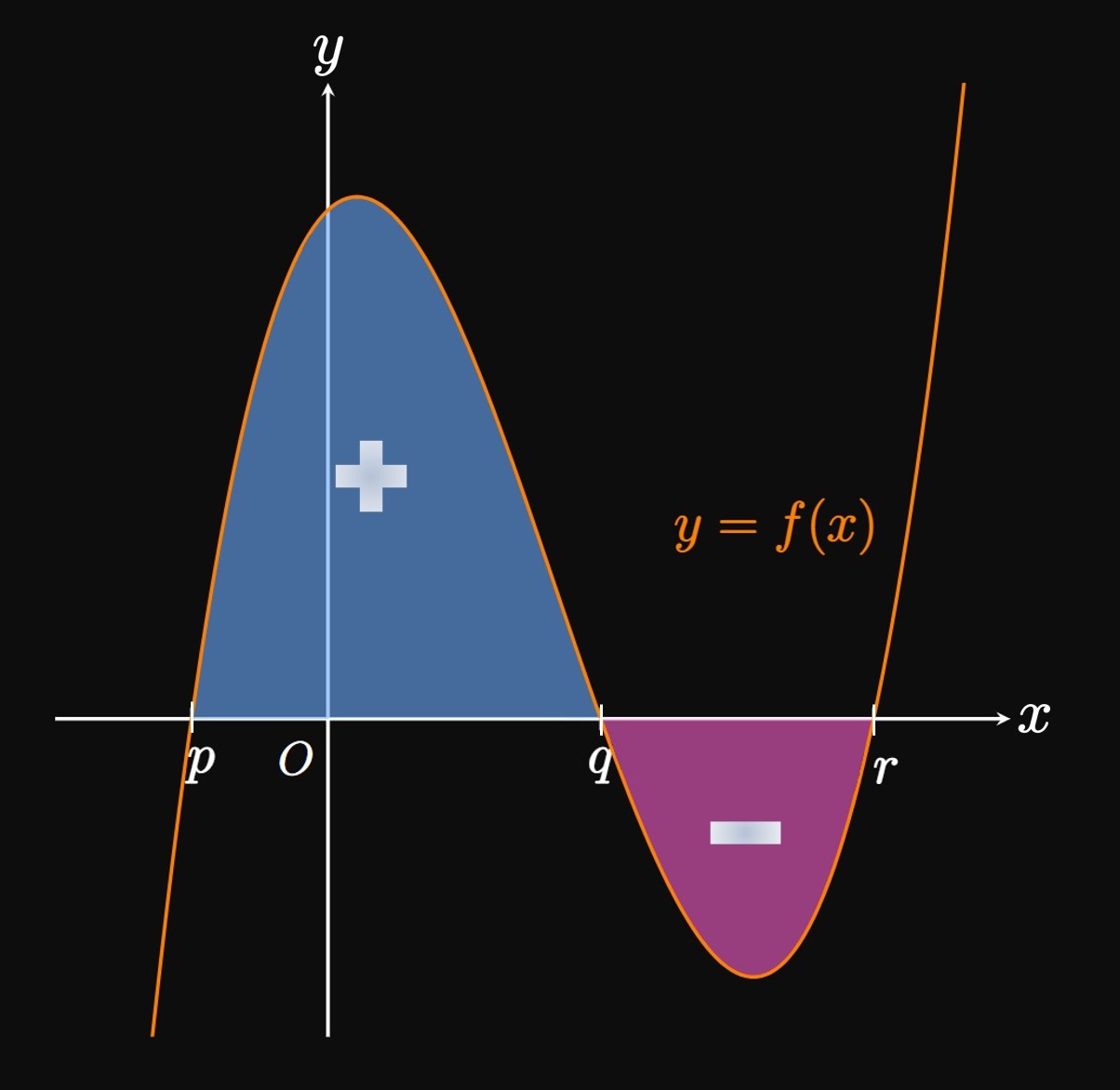
For example, in Figure 2 we see \(f(x) \geq 0\)
over \([p, q],\)
meaning \(\int_p^q f(x) \di x \gt 0.\)
(This region has positive area.
)
But \(f(x) \leq 0\) over \([q, r],\)
so \(\int_q^r f(x) \di x \lt 0.\)
(This region has negative area.
)
Integrating over the entire region \([p, r]\)
produces the net signed area of these regions; namely,
\[\int_p^r f(x) \di x = A_1 - A_2 \cma\]
where \(A_1\) is the area above the \(x\)-axis and \(A_2\) is the area below the \(x\)-axis.
- \(\ds \int_{-3}^3 \sqrt{9 - x^2} \di x\)
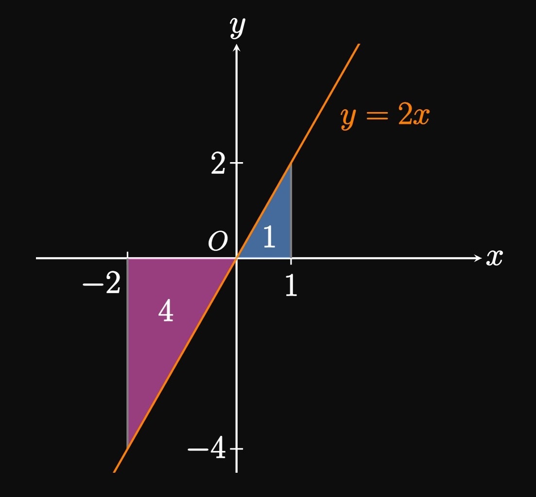
- \(\ds \int_{-2}^1 2x \di x\)
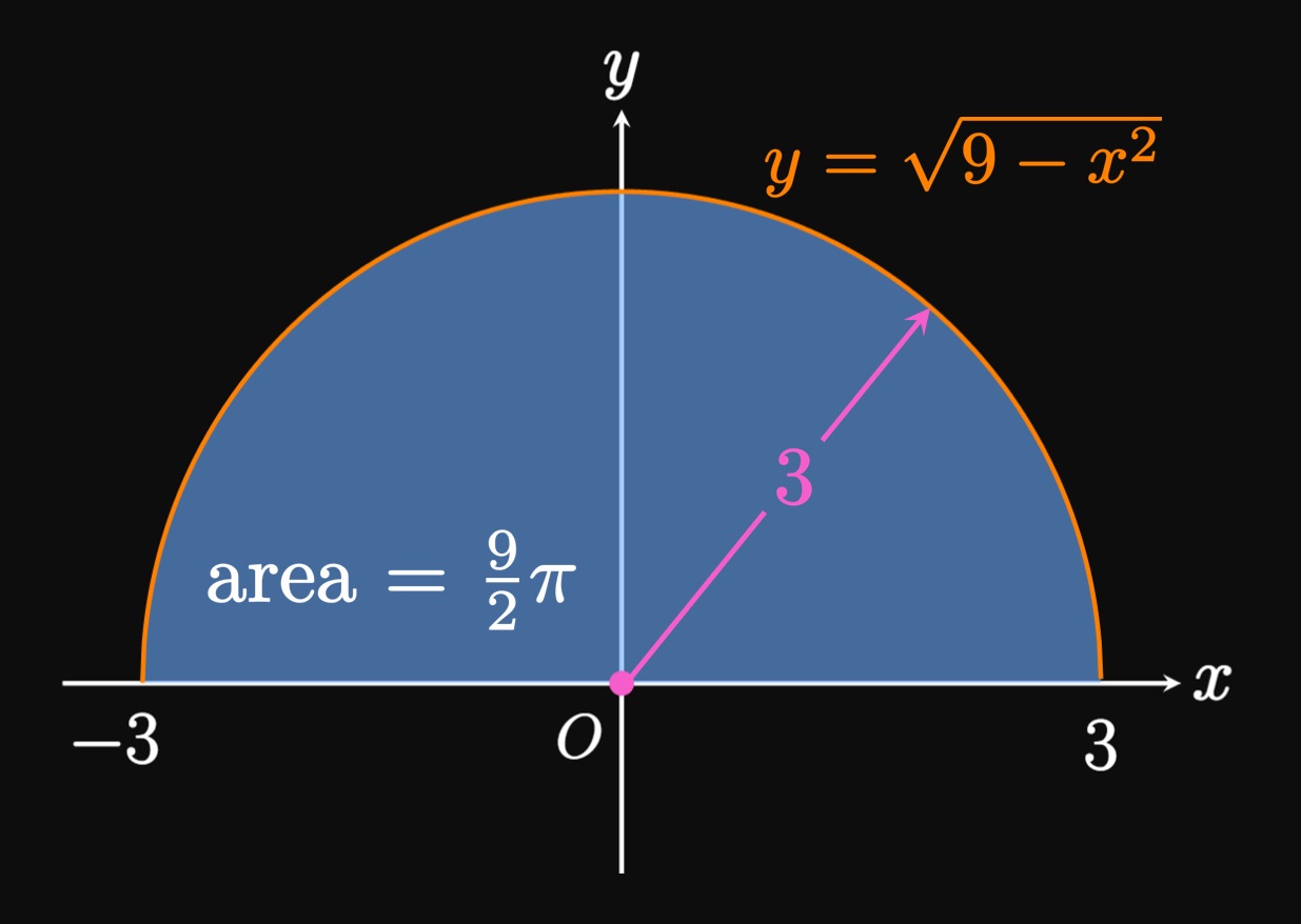
- The graph of \(y = \sqrt{9 - x^2}\) is a semicircle of radius \(3\) above the \(x\)-axis. The definite integral \(\int_{-3}^3 \sqrt{9 - x^2} \di x\) equals the entire area under the semicircle. Since the area of a circle of radius \(3\) is \(\pi(3)^2,\) a semicircle of radius \(3\) has half this area. Thus, \[\int_{-3}^3 \sqrt{9 - x^2} \di x = \tfrac{1}{2} \pi (3)^2 = \boxed{\tfrac{9}{2} \pi}\] (See Figure 3.)
-
The definite integral \(\int_{-2}^1 2x \di x\)
gives the net signed area bounded by the graph of \(y = 2x\)
and the \(x\)-axis between \(x = -2\) and \(x = 1.\)
The region under the \(x\)-axis (
negative area
) is a triangle of area \(4,\) whereas the region above the \(x\)-axis (positive area
) is a triangle of area \(1.\) So \[\int_{-2}^1 2x \di x = 1 - 4 = \boxed{-3}\] (See Figure 4.)
Evaluating Definite Integrals
Calculations often become easier if we select each sample point \(x_i^*\) to be the right endpoint \(x_i.\) Then \(\eqref{eq:A-int}\) becomes the right Riemann sum \begin{equation} \int_a^b f(x) \di x = \lim_{n \to \infty} \sum_{i = 1}^n f(x_i) \Delta x \cma \label{eq:A-int-right} \end{equation} where \(x_i = a + i \Delta x\) and \(\Delta x = (b - a)/n.\) But this Riemann sum isn't the only definition of \(\int_a^b f(x) \di x;\) it is merely a single, convenient definition. In many problems, we will use \(\eqref{eq:A-int-right}\) to calculate integrals.
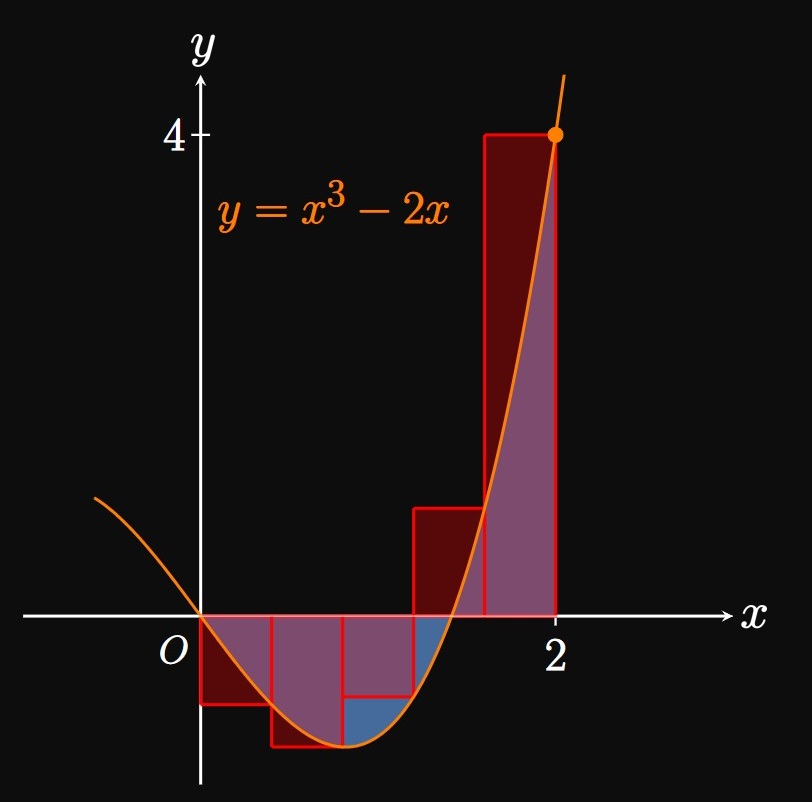
positive area) minus the area below the \(x\)-axis (the
negative area). Since our answer is positive, the Riemann sum estimates that the area above the \(x\)-axis is greater than the area below the \(x\)-axis. (See Figure 5.)
Summation Properties The following summation formulas are essential in evaluating limits as we compute definite integrals. If \(c\) is a constant, then the following relations hold: \begin{alignat}{2} &\sum_{i = 1}^n ca_i = c \sum_{i = 1}^n a_i \cma \label{eq:sum-c} \nl &\sum_{i = 1}^n c = c\,n \pd \label{eq:sum-cn} \nl \end{alignat} Observe that by \(\eqref{eq:sum-c},\) we can pull constants out of a summation expression; this is similar to how we can pull constants out of expressions in limits and derivatives. We also use the following formulas to deal with sums and differences in a summation expression: \begin{alignat}{2} &\sum_{i = 1}^n \par{a_i + b_i} &&= \sum_{i = 1}^n a_i + \sum_{i = 1}^n b_i \cma \label{eq:sum-sum} \nl &\sum_{i = 1}^n \par{a_i - b_i} &&= \sum_{i = 1}^n a_i - \sum_{i = 1}^n b_i \pd \label{eq:sum-difference} \nl \end{alignat} In words, the sum of addition or subtraction is the addition or subtraction of sums. As we evaluate limits to calculate definite integrals, we often work with sums of powers of positive integers, as we'll see in the following examples. Thus, the following formulas are critical: \begin{alignat}{2} &\sum_{i = 1}^n i &&= \frac{n(n + 1)}{2} \cma \label{eq:sum-i1} \nl &\sum_{i = 1}^n i^2 &&= \frac{n(n + 1)(2n + 1)}{6} \cma \label{eq:sum-i2} \nl &\sum_{i = 1}^n i^3 &&= \parbr{\frac{n(n + 1)}{2}}^2 \pd \label{eq:sum-i3} \end{alignat}
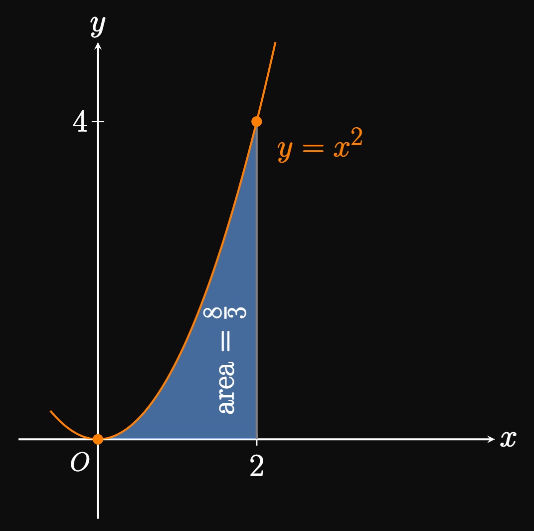
By comparison to \(\eqref{eq:A-int-right}\) we see \(a = 0,\) \(b = 3,\) and \(f(x) = x^3 - 3x^2 + 1.\) Thus, \[\Delta x = \frac{3 - 0}{n} = \frac{3}{n} \and x_i = 0 + i \Delta x = \frac{3i}{n} \pd\] Accordingly, \[ \ba \int_0^3 \par{x^3 - 3x^2 + 1} \di x &= \lim_{n \to \infty} \sum_{i = 1}^n f \par{\frac{3i}{n}} \frac{3}{n} \nl &= \lim_{n \to \infty} \frac{3}{n} \sum_{i = 1}^n f \par{\frac{3i}{n}} && [\text{by } \eqref{eq:sum-c}] \nl &= \lim_{n \to \infty} \frac{3}{n} \sum_{i = 1}^n \parbr{\par{\frac{3i}{n}}^3 - 3 \par{\frac{3i}{n}}^2 + 1} \nl &= \lim_{n \to \infty} \frac{3}{n} \parbr{\sum_{i = 1}^n \par{\frac{3i}{n}}^3 - 3 \sum_{i = 1}^n \par{\frac{3i}{n}}^2 + \sum_{i = 1}^n 1} &&[\text{by } \eqref{eq:sum-c}, \eqref{eq:sum-sum}, \text{and } \eqref{eq:sum-difference}] \nl &= \lim_{n \to \infty} \frac{3}{n} \parbr{\frac{27}{n^3} \sum_{i = 1}^n i^3 - \frac{27}{n^2} \sum_{i = 1}^n i^2 + \sum_{i = 1}^n 1} \pd && [\text{by } \eqref{eq:sum-c}] \ea \] To simplify the sums in the brackets, we apply \(\eqref{eq:sum-i3},\) \(\eqref{eq:sum-i2},\) and \(\eqref{eq:sum-cn}\) to each respective sum. Doing so shows \[ \ba \int_0^3 \par{x^3 - 3x^2 + 1} \di x &= \lim_{n \to \infty} \frac{3}{n} \parbr{\frac{27}{n^3} \par{\frac{n(n + 1)}{2}}^2 - \frac{27}{n^2} \cdot \frac{n(n + 1)(2n + 1)}{6} + n } \nl &= \lim_{n \to \infty} \frac{3}{n} \parbr{\frac{27(n + 1)^2}{4n} - \frac{9(n + 1)(2n + 1)}{2n} + n } \nl &= \lim_{n \to \infty} \parbr{\frac{81(n + 1)^2}{4n^2} - \frac{27(n + 1)(2n + 1)}{2n^2} + 3} \pd \ea \] To compute this limit with ease, we use the Sum and Difference Laws of Limits (see Section 1.2). Doing so and expanding each numerator give \[ \ba \int_0^3 \par{x^3 - 3x^2 + 1} \di x &= \parbr{\lim_{n \to \infty} \frac{81n^2 + 162n + 81}{4n^2}} - \parbr{\lim_{n \to \infty} \frac{54n^2 + 81n + 27}{2n^2}} + \parbr{\lim_{n \to \infty} 3} \nl &= \frac{81}{4} - 27 + 3 \nl &= \boxed{-\frac{15}{4}} \ea \]
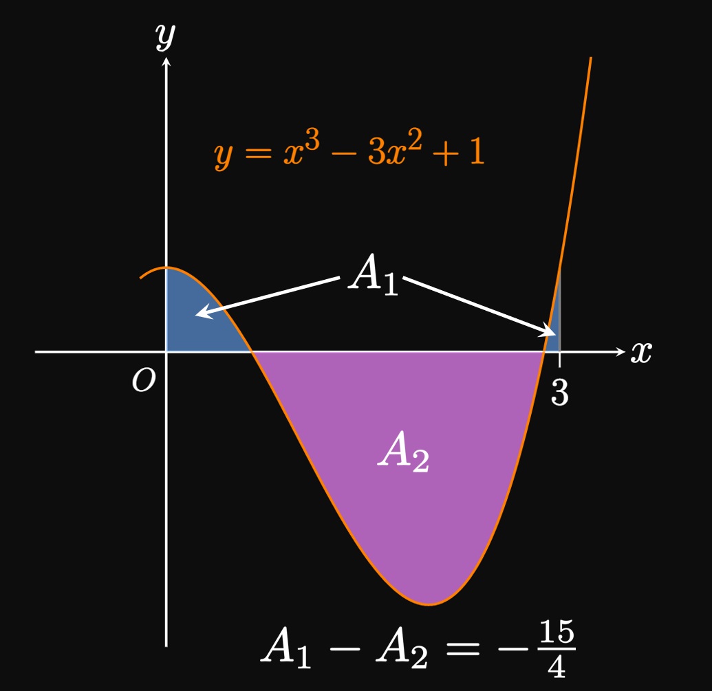
We interpret this result as follows: Over \(0 \leq x \leq 3\) let \(A_1\) be the total area bounded by \(y = x^3 - 3x^2 + 1\) above the \(x\)-axis, and let \(A_2\) be the area bounded by \(y = x^3 - 3x^2 + 1\) below the \(x\)-axis. Since \(A_1\) is positive and \(A_2\) is negative, the definite integral \(\int_0^3 \par{x^3 - 3x^2 + 1} \di x\) yields the net signed area \(A_1 - A_2.\) So \[ \int_0^3 \par{x^3 - 3x^2 + 1} \di x = A_1 - A_2 = -\frac{15}{4} \pd \] Because this result is negative, the area of the region below the \(x\)-axis is larger than the combined areas of the regions above the \(x\)-axis. (See Figure 7.)
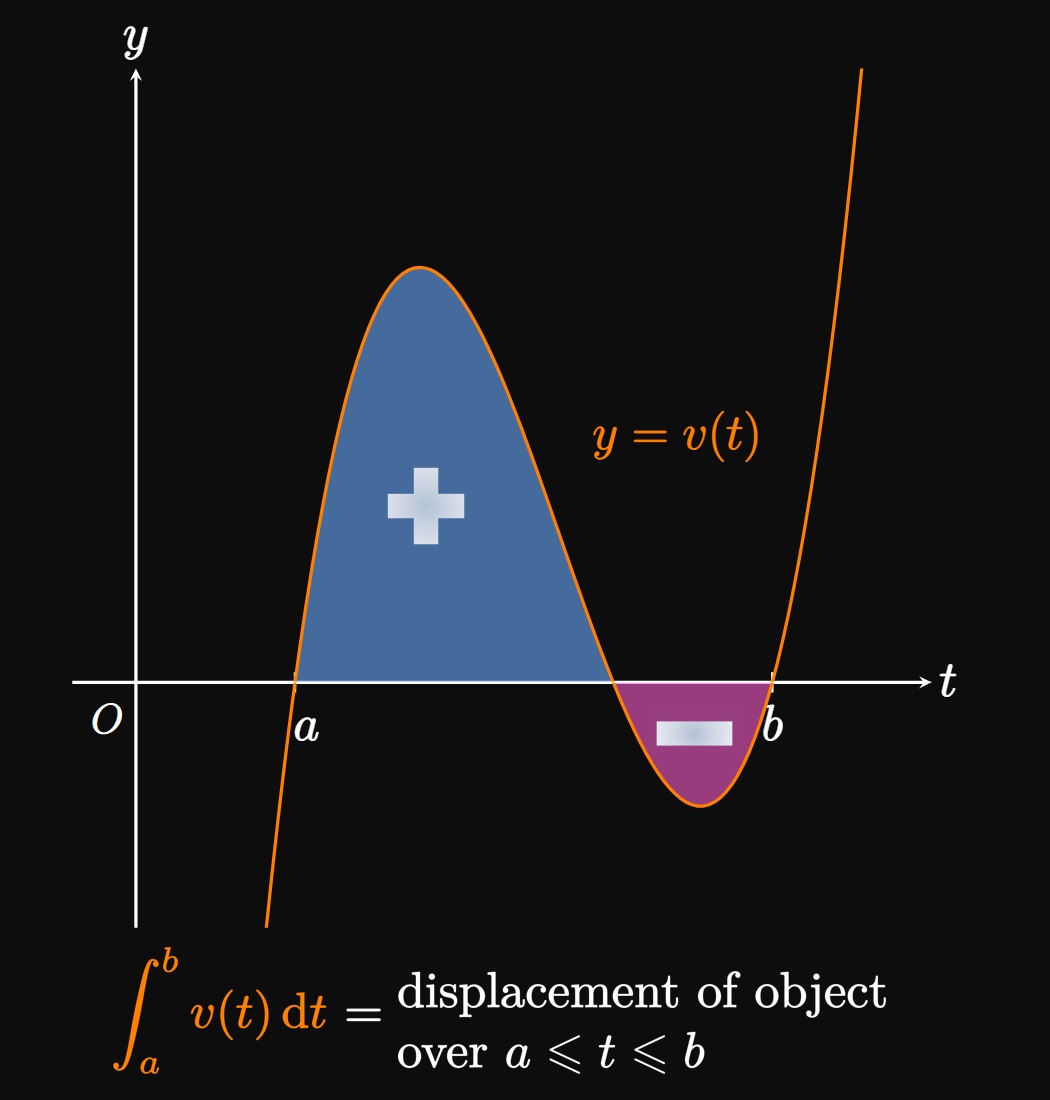
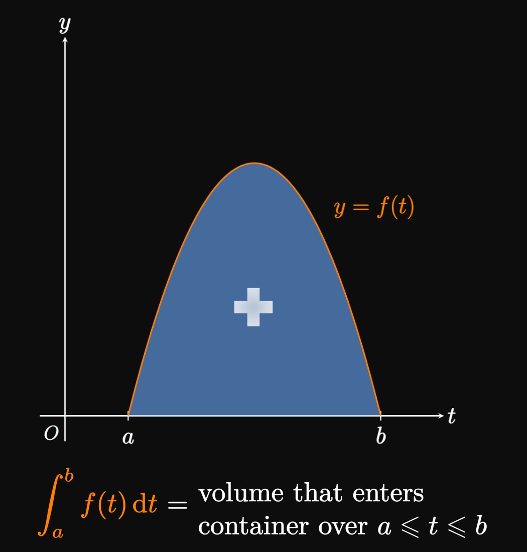
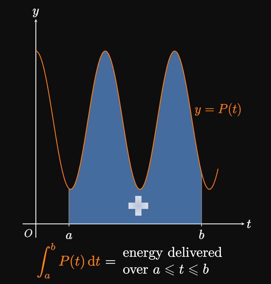
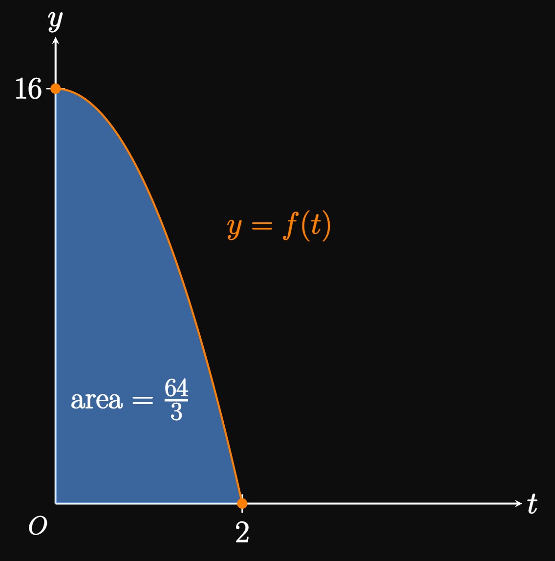
Applications of Integrals Definite integrals have more applications than simply calculating areas of arcane shapes. The area bounded by a curve is an extremely useful quantity in accumulation. For example, suppose that a particle travels along a straight line with velocity \(v\) as a function of time \(t.\) Then the net area bounded between the curve \(y = v(t)\) and the \(t\)-axis over \(a \leq t \leq b\) gives the particle's displacement. (See Figure 8A.) Likewise, if water enters a container with flow rate \(y = f(t),\) then the area under the curve \(f\) from \(a\) to \(b\) gives the volume of water that flows in over \(a \leq t \leq b.\) (See Figure 8B.) And if a power grid outputs power with time according to the function \(y = P(t),\) then the area under \(P\) from \(a\) to \(b\) represents the energy delivered over \(a \leq t \leq b,\) as shown by Figure 8C. Of course, countless more applications exist. Integral calculus is fundamental to nearly every scientific field; we'll discuss more uses in later sections.
Properties of Definite Integrals
In earlier chapters, we saw that it was very useful to develop properties for limits and derivatives. Similarly, we find great utility in properties of definite integrals.
Manipulating \(\Delta x\) Let \(f\) be an integrable function on some interval \([a, b].\) In Defining a Definite Integral, we defined \(\int_a^b f(x) \di x\) such that \(a \lt b.\) But if \(a \gt b,\) then the integral is still valid. Reversing \(a\) and \(b\) causes \(\Delta x\) to be \((a - b)/n,\) so \(\eqref{eq:A-int}\) becomes \[ \ba \int_b^a f(x) \di x &= \lim_{n \to \infty} \sum_{i = 1}^n f(x_i^*) \par{-\Delta x} \nl &= - \lim_{n \to \infty} \sum_{i = 1}^n f(x_i^*) \Delta x \nl &= - \int_a^b f(x) \di x \pd \ea \] Thus, we attain the general formula \begin{equation} \int_b^a f(x) \di x = -\int_a^b f(x) \di x \pd \label{eq:int-bounds-reversed} \end{equation} This property allows us to switch the bounds of integration if we tack on a negative sign. If \(a = b,\) then we see \begin{flalign} &&\Delta x = \frac{(a) - a}{n} &= 0 \cma \nonum &\nl \laWord{so} && \int_a^a f(x) \di x &= 0 \pd \label{eq:int-a-a} \end{flalign}
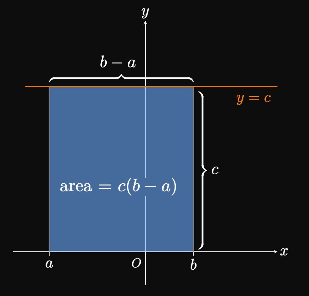
Integrals with Constants Just as we can pull a constant out of a derivative expression, we can pull a constant out of a definite integral. If \(f\) is integrable on \([a, b]\) and \(c\) is a constant, then \begin{equation} \int_a^b cf(x) \di x = c \int_a^b f(x) \di x \pd \label{eq:int-c} \end{equation} This formula is called the Constant Multiple Rule for Integrals. Since multiplying a function by \(c\) stretches or shrinks its graph by a factor \(c,\) each approximating rectangle's height is also stretched or shrunk by the factor \(c.\) If \(f(x) \geq 0,\) then the area under \(cf\) is \(c\) times the area under \(f.\) A similar geometric argument provides us the property \begin{equation} \int_a^b c \di x = c (b - a) \cma \label{eq:int-c-rectangle} \end{equation} called the Constant Rule for Integrals. Figure 10 shows a geometric interpretation of \(\eqref{eq:int-c-rectangle} \col\) For positive \(c,\) the area under the line \(y = c\) from \(x = a\) to \(x = b\) is a rectangle of height \(c\) and width \((b - a).\) Its area is therefore \(c(b - a).\) Observe that if \(c = 1,\) then \(\eqref{eq:int-c-rectangle}\) becomes \(\int_a^b \di x = b - a.\) In this case the integrand, despite appearing to be missing, is \(1.\)
PROOF OF \(\eqref{eq:int-c}\) Let's treat \(cf(x)\) as a single integrable function on \([a, b].\) Then by \(\eqref{eq:A-int},\) we have \[ \int_a^b cf(x) \di x = \lim_{n \to \infty} \sum_{i = 1}^n c f(x_i^*) \Delta x \pd \] Using \(\eqref{eq:sum-c}\) enables us to pull the constant \(c\) out of the summation function, and the Constant Multiple Law for Limits enables us to take \(c\) out of the limit expression. Doing so shows \[ \ba \int_a^b cf(x) \di x &= \lim_{n \to \infty} c \sum_{i = 1}^n f(x_i^*) \Delta x \nl &= c \lim_{n \to \infty} \sum_{i = 1}^n f(x_i^*) \Delta x \nl &= c \int_a^b f(x) \di x \pd \ea \] \[\qedproof\]
PROOF OF \(\eqref{eq:int-c-rectangle}\) If we let \(f(x) = c,\) then we see \(f(x_i^*) = c\) because the line \(y = c\) is uniform. Accordingly, \(\eqref{eq:A-int}\) gives \[ \int_a^b c \di x = \lim_{n \to \infty} \sum_{i = 1}^n c \Delta x \pd \] Applying \(\eqref{eq:sum-c}\) permits us to pull the \(c\) out of the summation expression; the Constant Multiple Law for Limits allows us to take \(c\) out of the limit. We see \[ \int_a^b c \di x = \lim_{n \to \infty} c \sum_{i = 1}^n \Delta x = c \lim_{n \to \infty} \sum_{i = 1}^n \Delta x \pd \] By \(\eqref{eq:sum-cn},\) the last step becomes \[ \int_a^b c \di x = c \, n \Delta x = c \, n \cdot \frac{b - a}{n} = c(b - a) \pd \] \[\qedproof\]
Integrals of Sums and Differences Properties of integrals are very similar to properties of derivatives. Let \(f\) and \(g\) be integrable functions over an interval \([a, b].\) Then \begin{flalign} &&\int_a^b \parbr{f(x) + g(x)} \di x &= \int_a^b f(x) \di x + \int_a^b g(x) \di x \label{eq:int-sum} &\nl \laWord{and} && \int_a^b \parbr{f(x) - g(x)} \di x &= \int_a^b f(x) \di x - \int_a^b g(x) \di x \pd \label{eq:int-difference} \end{flalign} We call these properties the Sum Rule for Integrals and the Difference Rule for Integrals, respectively. For positive functions, \(\eqref{eq:int-sum}\) asserts that the area under the curve \(f + g\) is the area under \(f\) plus the area under \(g.\) And \(\eqref{eq:int-difference}\) states that the area under \(f - g\) is the area under \(f\) minus the area under \(g.\)
PROOF OF \(\eqref{eq:int-sum}\) AND \(\eqref{eq:int-difference}\) Using \(\eqref{eq:A-int},\) the Riemann sum for the integral of \(f + g\) on \([a,b]\) is given by \[ \ba \int_a^b [f(x) + g(x)] \di x &= \lim_{n \to \infty} \sum_{i = 1}^n \parbr{f(x_i^*) + g(x_i^*)} \Delta x \nl &= \lim_{n \to \infty} \sum_{i = 1}^n f(x_i^*) \Delta x + \lim_{n \to \infty} \sum_{i = 1}^n g(x_i^*) \Delta x &&[\text{by } \eqref{eq:sum-sum}] \nl &= \int_a^b f(x) \di x + \int_a^b g(x) \di x \pd &&[\text{by } \eqref{eq:A-int}] \ea \] The proof for \(\eqref{eq:int-difference}\) is nearly identical. The Riemann sum for the integral of \(f - g\) on \([a,b]\) is given by \[ \ba \int_a^b [f(x) - g(x)] \di x &= \lim_{n \to \infty} \sum_{i = 1}^n \parbr{f(x_i^*) - g(x_i^*)} \Delta x \nl &= \lim_{n \to \infty} \sum_{i = 1}^n f(x_i^*) \Delta x - \lim_{n \to \infty} \sum_{i = 1}^n g(x_i^*) \Delta x &&[\text{by } \eqref{eq:sum-difference}] \nl &= \int_a^b f(x) \di x - \int_a^b g(x) \di x \pd &&[\text{by } \eqref{eq:A-int}] \ea \] \[\qedproof\]

We introduce a final property that enables us to merge integrals of the same function \(f\) over adjacent intervals. If \(c\) is a constant and \(f\) is integrable over \([a, b],\) \([a, c],\) and \([c, b],\) then \begin{equation} \int_a^b f(x) \di x = \int_a^c f(x) \di x + \int_c^b f(x) \di x \pd \label{eq:int-adj} \end{equation} For the special case \(f(x) \geq 0\) and \(a \lt c \lt b,\) \(\eqrefer{eq:int-adj}\) asserts that the area under \(f\) over \([a, c]\) plus the area under \(f\) over \([c, b]\) equals the area under \(f\) over \([a, b].\) Think of the line \(x = c\) splitting the region under \(f\) over \([a, b].\) (See Figure 11.)
Comparison Properties of Definite Integrals
Let's discuss some properties to help us infer the value of a definite integral. We begin with the simplest property. If \(f(x)\) is integrable over \([a, b]\) and \(f(x) \geq 0,\) then the region bounded by \(f\) is above the \(x\)-axis. Thus, \begin{equation} \int_a^b f(x) \di x \geq 0 \pd \label{eq:int-prop-pos} \end{equation} This form is simple yet powerful in making inferences. If we can show that a function is positive, then its area—which can represent physical quantities such as displacement, volume, and energy—must be positive and related to the function. (We will explore this relationship in Section 4.3.)
If \(f\) and \(g\) are integrable functions over \([a, b]\) such that \(f(x) \geq g(x)\) for \(a \leq x \leq b,\) then \begin{equation} \int_a^b f(x) \di x \geq \int_a^b g(x) \di x \pd \label{eq:int-inequality} \end{equation} In words, a larger function has a larger integral. Thus, inequalities are preserved when we take definite integrals. If \(f(x) \geq 0\) and \(g(x) \geq 0\) over \([a, b],\) then \(f\) encloses a larger region than \(g\) and so the area under \(f\) is greater than the area under \(g.\)
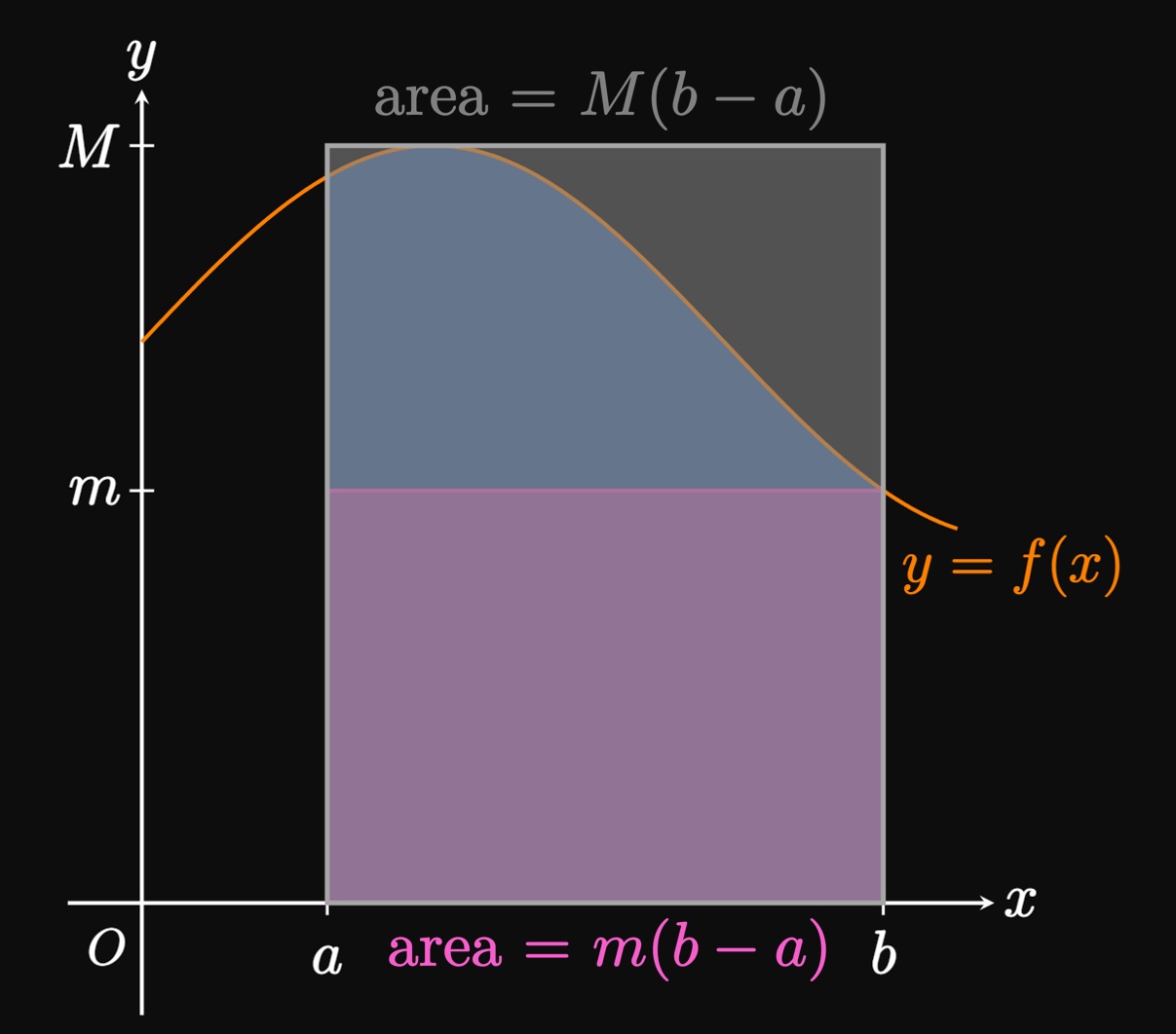
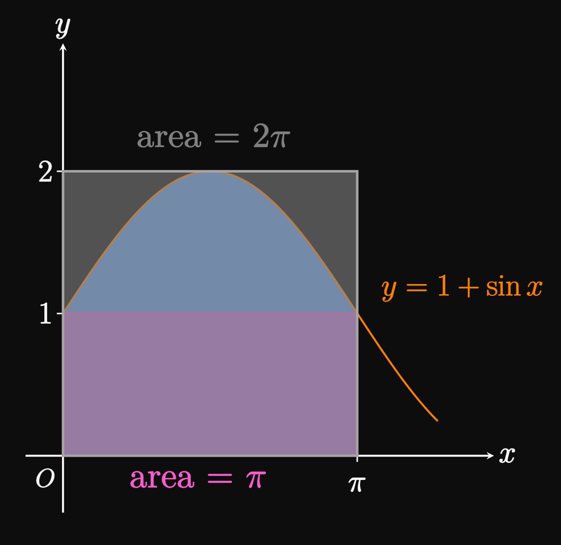
The final property we discuss allows us to bound an integral—that is, prove that its value lies between two numbers. If \(m \leq f(x) \leq M\) for \(a \leq x \leq b,\) then \(\eqref{eq:int-inequality}\) gives \[\int_a^b m \di x \leq \int_a^b f(x) \di x \leq \int_a^b M \di x \pd\] We use \(\eqref{eq:int-c-rectangle}\) to evaluate the left- and right-bounding integrals; the inequality therefore becomes \begin{equation} m(b - a) \leq \int_a^b f(x) \di x \leq M(b - a) \pd \label{eq:int-prop-bounds} \end{equation} If \(f(x) \geq 0,\) then this formula asserts that \(\int_a^b f(x) \di x\) is greater than the area of a rectangle of height \(m\) but less than the area of a rectangle of height \(M.\) (See Figure 12.) This property is especially useful if we choose \(m\) and \(M\) to be the absolute minimum and absolute maximum values, respectively, of \(f\) over \([a, b].\)
- If \(f(x) \geq 0\) for \(a \leq x \leq b,\) then \begin{equation} \int_a^b f(x) \di x \geq 0 \pd \eqlabel{eq:int-prop-pos} \end{equation}
- If \(f(x) \geq g(x)\) for \(a \leq x \leq b,\) then \begin{equation} \int_a^b f(x) \di x \geq \int_a^b g(x) \di x \pd \eqlabel{eq:int-inequality} \end{equation}
- If \(m \leq f(x) \leq M\) for \(a \leq x \leq b,\) then \begin{equation} m(b - a) \leq \int_a^b f(x) \di x \leq M(b - a) \pd \eqlabel{eq:int-prop-bounds} \end{equation}
Areas under Curves To estimate the area under a curve \(y = f(x),\) where \(f(x) \geq 0\) over \(a \leq x \leq b,\) we cut the region into many rectangles of width \(\Delta x = (b - a)/n.\) The sum of these rectangles is called a Riemann sum. As we increase \(n,\) \(\Delta x\) shrinks and more rectangles are inscribed under the curve. If we let \(n \to \infty,\) then a Riemann sum gives the exact area under a curve. Let \(a = x_0,\) \(x_1,\) \(\dots, x_{n - 1}, x_n = b\) be the endpoints of \(n\) equal-width subintervals, and let \(x_1^*, x_2^*,\) \(\dots, x_n^*\) be any sample points in these subintervals. Then \begin{equation} A = \lim_{n \to \infty} \sum_{i = 1}^n f(x_i^*) \Delta x \pd \eqlabel{eq:A-lim} \end{equation} If this limit exists and gives the same number \(A\) for all possible sample points \(x_i^*,\) then \(f\) is called integrable over \([a, b].\)
Defining a Definite Integral If \(f(x) \geq 0,\) then a definite integral \(\int_a^b f(x) \di x\) equals the area under the curve \(y = f(x)\) from \(x = a\) to \(x = b.\) The Riemann definition of a definite integral is given by \begin{equation} \int_a^b f(x) \di x = \lim_{n \to \infty} \sum_{i = 1}^n f(x_i^*) \Delta x \pd \eqlabel{eq:A-int} \end{equation} A definite integral yields a positive number if the region is above the \(x\)-axis but a negative number if the region is below the \(x\)-axis. If we integrate over an interval \([a, b]\) in which some regions are above the \(x\)-axis and some regions are below, then the definite integral returns the net signed area—namely, \[\int_a^b f(x) \di x = A_1 - A_2 \cma\] where \(A_1\) is the area above the \(x\)-axis and \(A_2\) is the area below the \(x\)-axis.
Evaluating Definite Integrals It is convenient to pick sample points such that \(x_i^* = x_i.\) If \(f\) is integrable on \([a, b],\) then \begin{equation} \int_a^b f(x) \di x = \lim_{n \to \infty} \sum_{i = 1}^n f(x_i) \Delta x \cma \eqlabel{eq:A-int-right} \end{equation} where \[\Delta x = \frac{b - a}{n} \and x_i = a + i \Delta x \pd\] This form is an easy way to compute many definite integrals.
Properties of Definite Integrals We have a few special definitions for definite integrals. If \(f\) is integrable on \([a, b],\) then \begin{equation} \int_b^a f(x) \di x = -\int_a^b f(x) \di x \pd \eqlabel{eq:int-bounds-reversed} \end{equation} If \(f\) is defined at \(a,\) then \[\int_a^a f(x) \di x = 0 \pd \eqlabel{eq:int-a-a}\] Properties with integrals are similar to properties with derivatives. Let \(c\) be a constant, and let \(f\) be an integrable function over \([a, b].\) Then \begin{align} &\int_a^b cf(x) \di x = c \int_a^b f(x) \di x \cma &&[\text{Constant Multiple Rule}] \eqlabel{eq:int-c} \nl &\int_a^b c \di x = c (b - a) \pd &&[\text{Constant Rule}] \eqlabel{eq:int-c-rectangle} \end{align} If \(f\) and \(g\) are integrable functions on \([a, b],\) then \begin{align} \int_a^b \parbr{f(x) + g(x)} \di x &= \int_a^b f(x) \di x + \int_a^b g(x) \di x \cma &&[\text{Sum Rule}] \eqlabel{eq:int-sum} \nl \int_a^b \parbr{f(x) - g(x)} \di x &= \int_a^b f(x) \di x - \int_a^b g(x) \di x \pd &&[\text{Difference Rule}] \eqlabel{eq:int-difference} \end{align} The Additive Interval Property asserts that if \(c\) is a constant and \(f\) is integrable over \([a, b],\) \([a, c],\) and \([c, b],\) then \begin{equation} \int_a^b f(x) \di x = \int_a^c f(x) \di x + \int_c^b f(x) \di x \pd \eqlabel{eq:int-adj} \end{equation}
Comparison Properties of Definite Integrals Comparison properties enable us to infer values of definite integrals. In general, inequalities are conserved when we take definite integrals, as shown by the following properties.
- If \(f(x) \geq 0\) for \(a \leq x \leq b,\) then \begin{equation} \int_a^b f(x) \di x \geq 0 \pd \eqlabel{eq:int-prop-pos} \end{equation}
- If \(f(x) \geq g(x)\) for \(a \leq x \leq b,\) then \begin{equation} \int_a^b f(x) \di x \geq \int_a^b g(x) \di x \pd \eqlabel{eq:int-inequality} \end{equation}
- If \(m \leq f(x) \leq M\) for \(a \leq x \leq b,\) then \begin{equation} m(b - a) \leq \int_a^b f(x) \di x \leq M(b - a) \pd \eqlabel{eq:int-prop-bounds} \end{equation}